This post presents a framework to help you quickly transform your soil profiles observations into a graph, with R and {ggplot2}. For soil and horizons names, we will use the terminology defined by the World reference base for soil resources (FAO, 2014).
The world reference base for soil resources (WRB) comprises two levels of categorical detail:
- First level: 32 reference soil groups
- Second level: name of the reference soil groups combined with a set of principal and supplementary qualifiers.
For this tutorial, we will use only the first level and only refers to some of the main soil groups.
1. Plotting one soil profile
Let’s start with a simple description of a calcisol. As a minimal example, the field notes related to one soil profile can be summarized as follows:
# Calcisol description
soil_profile <- cbind.data.frame(
  profile = "Calcisol",               # Name of the whole profil
  from = c(0,0.2),                    # Beginning of each horizon
  to = c(0.2,0.4),                    # End of each horizon
  horizon=c('Mollic','Calcic'),       # Name of the horizon
  munsell=c('10YR 3/2','10YR 7/2')    # Munsell color (Page, followed by value, then chroma)
)

soil_profile
## profile from to horizon munsell
## 1 Calcisol 0.0 0.2 Mollic 10YR 3/2
## 2 Calcisol 0.2 0.4 Calcic 10YR 7/2Before making our first plot, we will do some data manipulation. To do so, we will load the {tidyverse} extension, which also includes {ggplot2} (you may refer to this post for more information about the {tidyverse}).
library(tidyverse)Using tidy syntax, we will add a new column to specify each horizon height on our original data frame.
# Calcisol description
soil_profile <- soil_profile%>%
  mutate(
    height = to - from
  )

soil_profile
## profile from to horizon munsell height
## 1 Calcisol 0.0 0.2 Mollic 10YR 3/2 0.2
## 2 Calcisol 0.2 0.4 Calcic 10YR 7/2 0.2Now we are ready to make our first plot, using geom_col to represent our soil profile.
soil_plot<-ggplot(
  data = soil_profile,
  aes(
    x=profile,y=-height,                       # specify x and y axis
    fill=fct_reorder(horizon,to,.desc=TRUE))   # make sure that horizons are on the right order
  )+
  geom_col(
    width=0.4                                  # Profile width
  )

soil_plot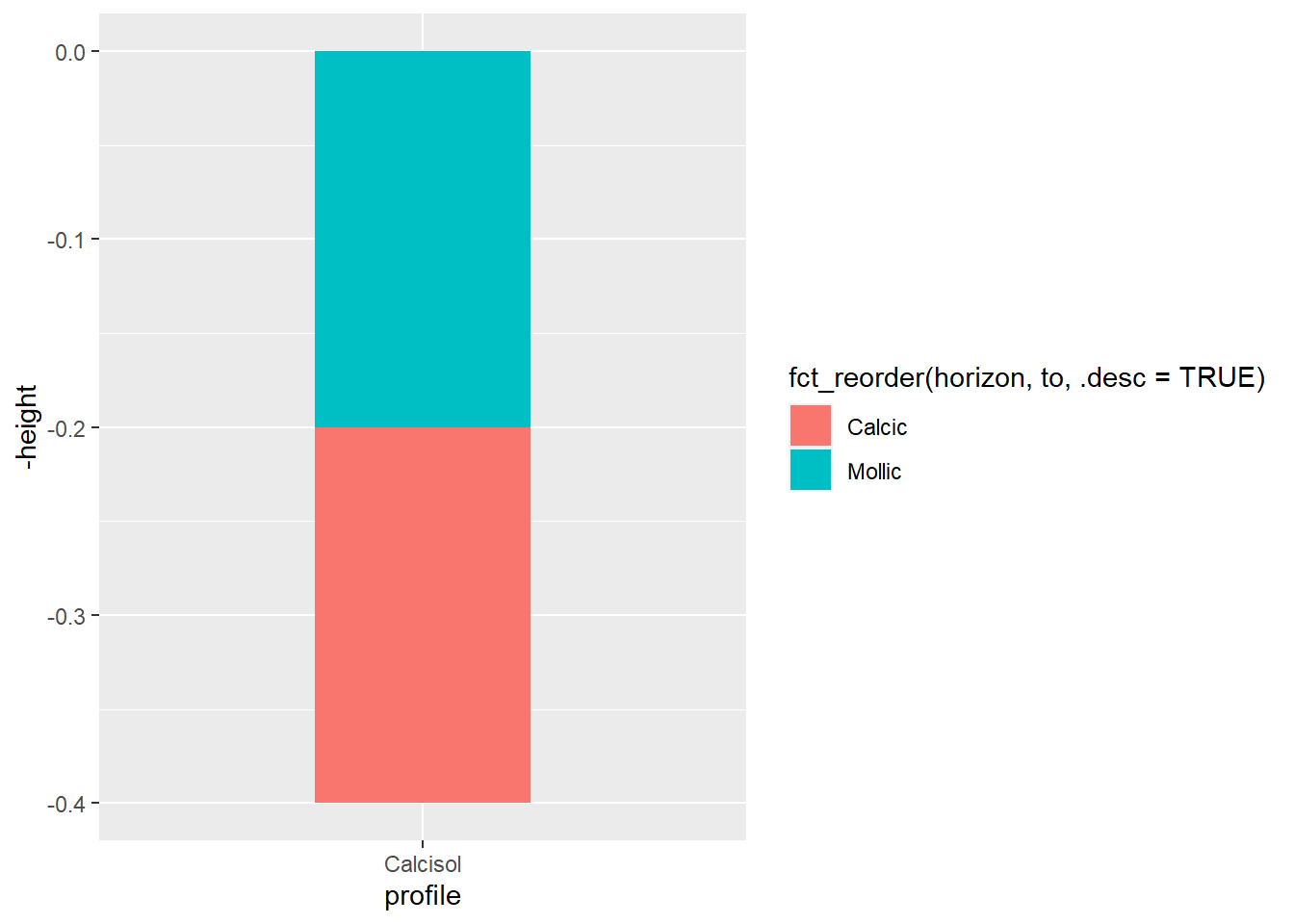
If you are not familiar with {ggplot2} syntax, you may read this tutorial for more information. In the following lines, we will detail more closely certain particularities related to soil profiles representations.
One of the first thing we want to change in our plot is the horizon colors to match field observations.
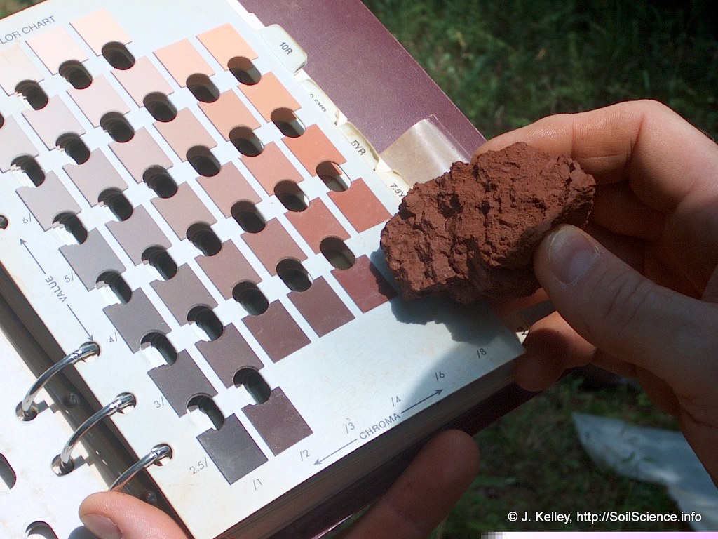
Figure 1 The Munsell soil color charts (Image credit: SoilScience.info)
Munsell notations are not directly readable in R. Fortunately, the {munsell} extension developed by Charlotte Wickham allows to transform Munsell notations into hex code, which are usable in R. A small drawback is that this extension only works for even chroma, whereas we also have odd chromas inside the Munsell soil color charts we use on the fields (soil scientists love precision!).
# Install extension (to do only once)
#install.packages('munsell')
# Load extension
library(munsell)  # Only works for even chroma
Now that we loaded the {munsell} extension, we may plot some colors with plot_mnsl.
plot_mnsl("10YR 2/2")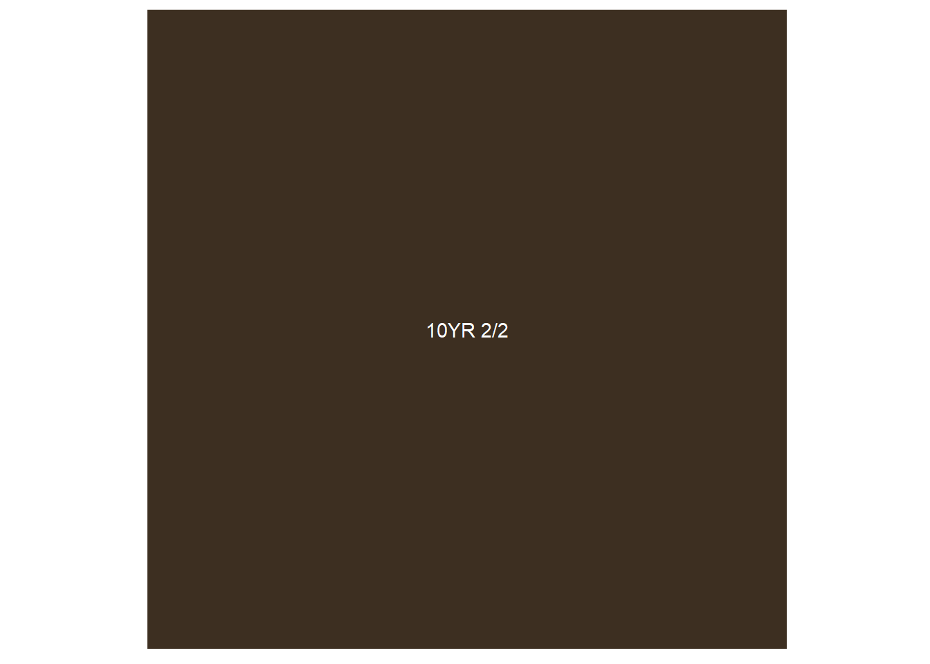
However, the function we are most interested in is mnsl(), to convert Munsell notations to hex color codes.
mnsl("10YR 2/2")## [1] "#3D2F21"Using this function, we will add a new column to our dataframe with the hex code matching the Munsell notation.
soil_profile<-soil_profile%>%
  mutate(hex=mnsl(munsell))

soil_profile
## profile from to horizon munsell height hex
## 1 Calcisol 0.0 0.2 Mollic 10YR 3/2 0.2 #554636
## 2 Calcisol 0.2 0.4 Calcic 10YR 7/2 0.2 #BEAD98Now we are ready to use this information to represent the real horizon colors on our plot.
soil_plot<-soil_plot+
  scale_fill_manual(
    breaks=soil_profile$horizon,
    values=soil_profile$hex)

soil_plot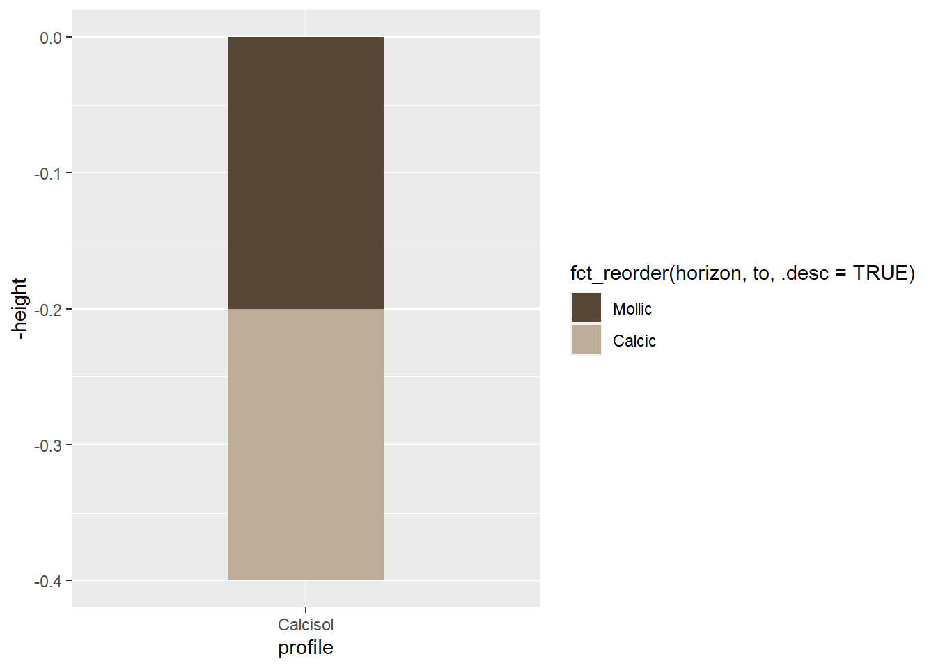
Next step is to add the names of the horizons directly on the plot (and not in the legend next to it). We will do so with geom_text, taking advantage of the height column we created before.
soil_plot<-soil_plot+
  guides(fill=FALSE)+                      # Hide legend
  geom_text(
    aes(y=-(from+height/2),label=horizon)  # Insert horizon names on the plot
  )

soil_plot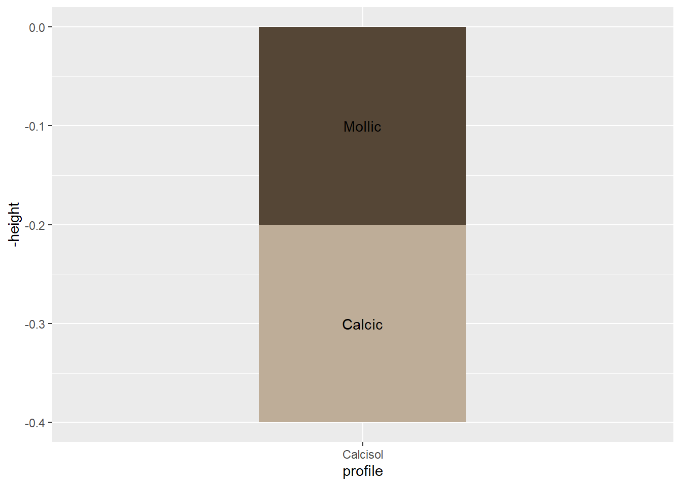
We may now finish our first plot with some customization.
soil_plot+
  scale_x_discrete(position = "top")+    # Move profile name to the top
  labs(
    title = "Soil profile description",
    y = "Depth (meters)",
    x=""
  )+
  theme_minimal()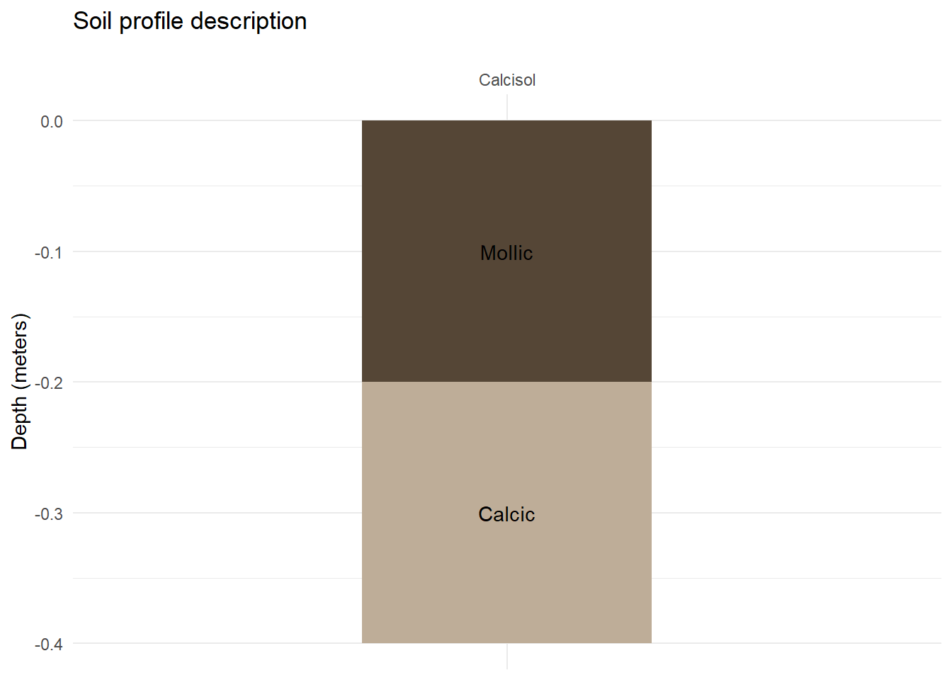
2. Plotting a soil chronosequence
Starting from this example, we will now see how we can plot a soil chronosequence. With the continuation of rock alteration and the leaching of the carbonates, calcisol may evolve into cambisol. Cambisols show signs of soil evolution such as colour change, soil structure development or leaching of carbonates but lack sufficient soil evolution to be included in other reference soil groups.
# Calcisol description
calcisol <- cbind.data.frame(
  profile = "Calcisol",
  from = c(0,0.2),
  to = c(0.2,0.4),
  horizon=c('Mollic','Calcic'),
  munsell=c('10YR 3/2','10YR 7/2')
)

# Cambisol description
cambisol <- cbind.data.frame(
  profile = "Cambisol",
  from = c(0,0.2),
  to = c(0.2,0.8),
  horizon=c('Mollic','Cambic'),
  munsell=c("10YR 3/2","10YR 5/2") # First value, then chroma
)

# Merging profiles observation
soil_profile <- rbind.data.frame(
  calcisol,
  cambisol
)

# Adding height & hex colors
soil_profile <- soil_profile%>%
  mutate(
    height = to - from
  )%>%
  mutate(hex=mnsl(munsell))

soil_profile
## profile from to horizon munsell height hex
## 1 Calcisol 0.0 0.2 Mollic 10YR 3/2 0.2 #554636
## 2 Calcisol 0.2 0.4 Calcic 10YR 7/2 0.2 #BEAD98
## 3 Cambisol 0.0 0.2 Mollic 10YR 3/2 0.2 #554636
## 4 Cambisol 0.2 0.8 Cambic 10YR 5/2 0.6 #897866Now that our dataframe is ready, we just have to follow excatly the same steps as previously to create a plot with multiple soil profiles.
soil_plot<-ggplot(
  data = soil_profile,
  aes(
    x=profile,y=-height,
    fill=fct_reorder(horizon,to,.desc=TRUE))
  )+
  geom_col(
    width=0.4
  )+
  scale_fill_manual(
    breaks=soil_profile$horizon,
    values=soil_profile$hex
  )+
  guides(fill=FALSE)+
  geom_text(
    aes(y=-(from+height/2),label=horizon),
    color="white",fontface="italic",size=3.5
  )+
  scale_x_discrete(position = "top")+
  labs(
    title = "Soil chronosequence",
    y = "Depth (meters)",
    x=""
  )+
  theme_minimal()

soil_plot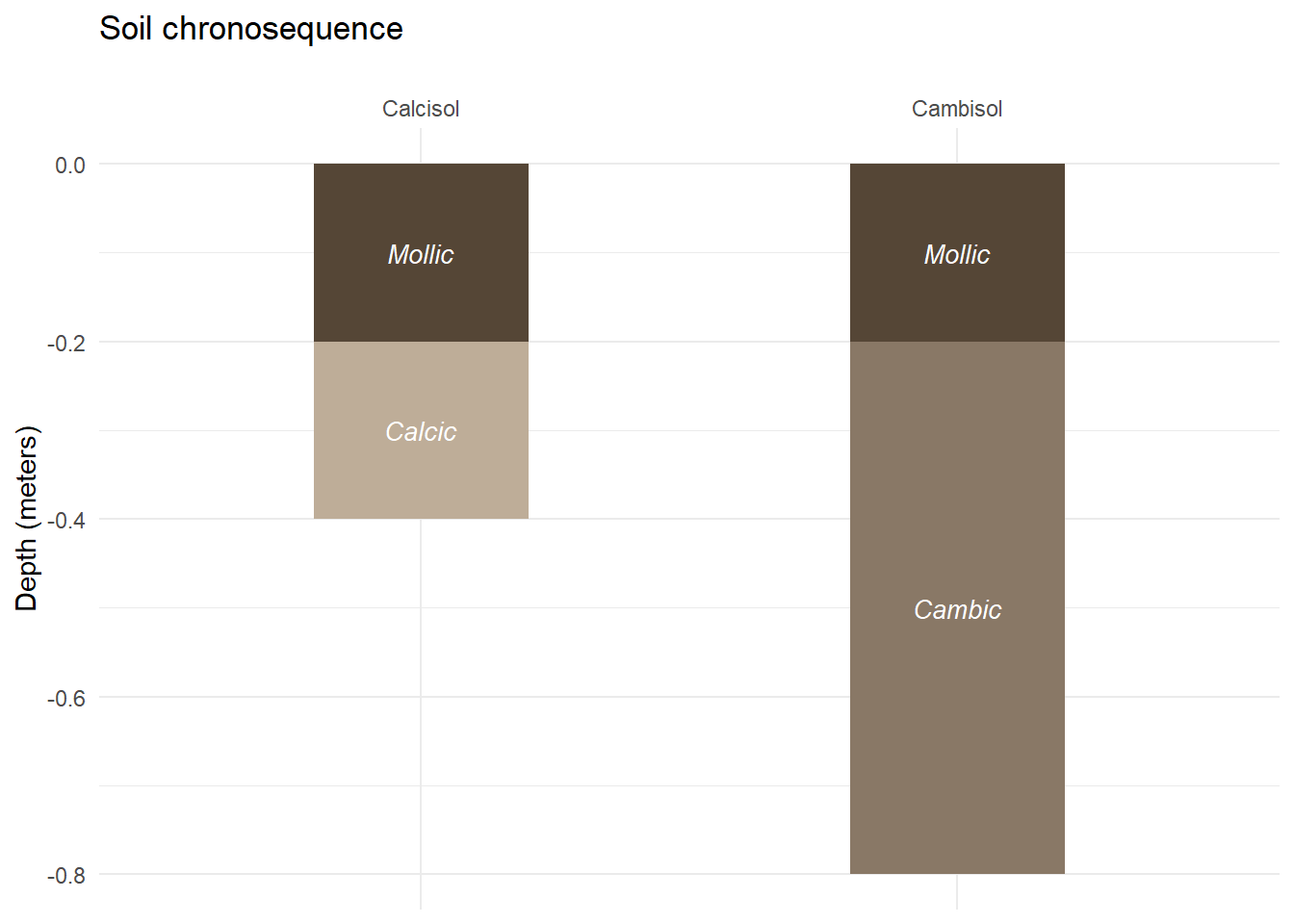
3. Finer description of horizons
We will now see how we can add additional information on the plot about the characteristics of the soil horizons and profiles.
First, we will add a new profile to our chronosequence: a luvisol. Luvisols have a higher clay content in the subsoil than in the topsoil, as a result of pedogenetic processes (especially clay migration) leading to an argic subsoil horizon, that comes underneath an eluvial albic horizon.
# Luvisol description
luvisol <- cbind.data.frame(
  profile = "Luvisol",
  from = c(0,0.2,0.4),
  to = c(0.2,0.4,0.9),
  horizon=c('Mollic','Albic','Argic'),
  munsell=c("10YR 1/2",'7.5YR 8/2',"10YR 3/2") # First value, then chroma
)

# Merging profiles observation
soil_profile <- rbind.data.frame(
  calcisol,
  cambisol,
  luvisol
)

# Adding height & hex colors
soil_profile <- soil_profile%>%
  mutate(
    height = to - from
  )%>%
  mutate(hex=mnsl(munsell))

soil_profile
## profile from to horizon munsell height hex
## 1 Calcisol 0.0 0.2 Mollic 10YR 3/2 0.2 #554636
## 2 Calcisol 0.2 0.4 Calcic 10YR 7/2 0.2 #BEAD98
## 3 Cambisol 0.0 0.2 Mollic 10YR 3/2 0.2 #554636
## 4 Cambisol 0.2 0.8 Cambic 10YR 5/2 0.6 #897866
## 5 Luvisol 0.0 0.2 Mollic 10YR 1/2 0.2 #291A0A
## 6 Luvisol 0.2 0.4 Albic 7.5YR 8/2 0.2 #DAC7B5
## 7 Luvisol 0.4 0.9 Argic 10YR 3/2 0.5 #554636Now we can follow the same steps as in the previous parts to make a first plot of this extended chronosequence.
soil_plot<-ggplot(
  data = soil_profile,
  aes(
    x=profile,y=-height,
    fill=fct_reorder(horizon,to,.desc=TRUE))
  )+
  geom_col(
    width=0.4
  )+
  scale_fill_manual(
    breaks=soil_profile$horizon,
    values=soil_profile$hex
  )+
  guides(fill=FALSE)+
  geom_text(
    aes(y=-(from+height/2),label=horizon),
    color="white",fontface="italic",size=3.5
  )+
  scale_x_discrete(position = "top")+
  labs(
    title = "Soil chronosequence",
    y = "Depth (meters)",
    x=""
  )+
  theme_minimal()

soil_plot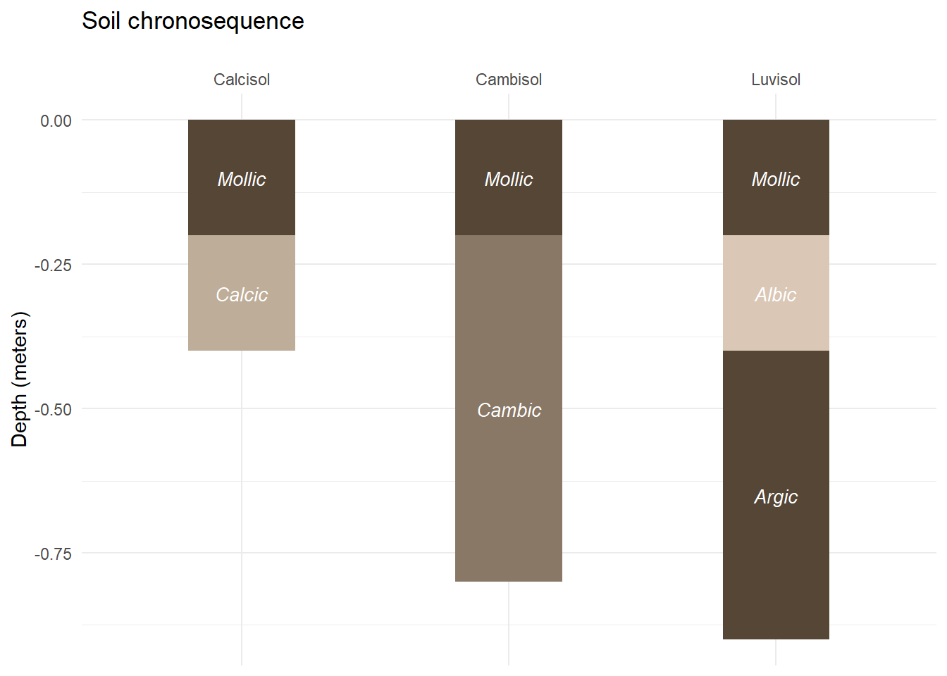
One of the frequent consequences of clay migration is the accumulation of water at depth, which leads to iron oxydation. So we expect to find red marks on the argic horizon, as sign of this oxidation.
Figure 2 Chromic luvisol with features associated with water stagnation in the argic horizon, China (Image credit: isric.org)
Let’s see how to add this information on our plot. We will start by adding a column to our dataframe to indicate on which horizon we have observed oxidation marks (normally, this information should have been directly present in our field observations, and therefore in our initial dataframe).
# Adding new column to specify that we only observed oxidation on the argic horizon
soil_profile <- soil_profile%>%
  mutate(
    oxy = case_when(
      horizon=="Argic"~"Yes",
      TRUE~"No"
    )
  )

soil_profile
## profile from to horizon munsell height hex oxy
## 1 Calcisol 0.0 0.2 Mollic 10YR 3/2 0.2 #554636 No
## 2 Calcisol 0.2 0.4 Calcic 10YR 7/2 0.2 #BEAD98 No
## 3 Cambisol 0.0 0.2 Mollic 10YR 3/2 0.2 #554636 No
## 4 Cambisol 0.2 0.8 Cambic 10YR 5/2 0.6 #897866 No
## 5 Luvisol 0.0 0.2 Mollic 10YR 1/2 0.2 #291A0A No
## 6 Luvisol 0.2 0.4 Albic 7.5YR 8/2 0.2 #DAC7B5 No
## 7 Luvisol 0.4 0.9 Argic 10YR 3/2 0.5 #554636 YesNow we will use the {ggpattern} extension from Mike FC to add a specific pattern to the horizon with oxidation marks.
# Install {ggpattern}
#remotes::install_github("coolbutuseless/ggpattern")
# Load {ggpattern}
library(ggpattern)
Many usual {ggplot2} geom_ may be used with {ggpattern}. Here we will simply change geom_col used previously for geom_col_pattern, so we can add patterns to our barplot.
soil_plot<-ggplot(
  data = soil_profile,
  aes(
    x=profile,y=-height
  ))+
  geom_col_pattern(                               # Changing geom_col to geom_col_pattern
    aes(
      fill=fct_reorder(horizon,to,.desc=TRUE),    # Moving fill form ggplot to this aes()
      pattern_fill=oxy                            # New pattern_fill attribute
    ),
    width=0.4,
    pattern_color=NA                              # Hide pattern outside borders
  )+
  scale_pattern_fill_manual(                      # Choose pattern colors
    values=c(NA,"indianred"),
    breaks=c("No","Yes")
  )

soil_plot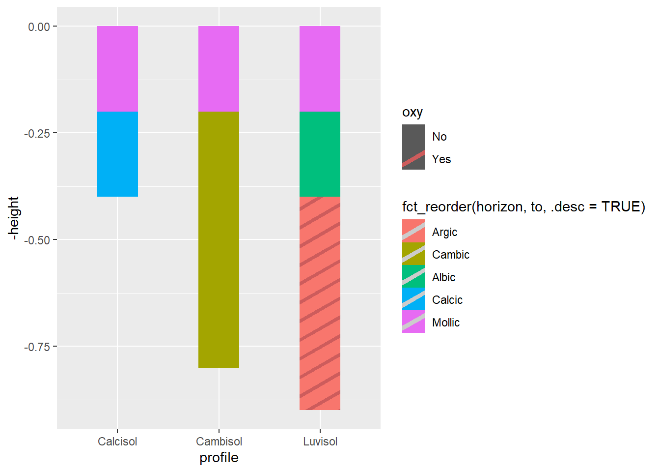
Now that we have seen how geom_col_pattern works, we can add former customization to our new plot.
soil_plot<-soil_plot+
  scale_fill_manual(
    breaks=soil_profile$horizon,
    values=soil_profile$hex
  )+
  guides(
    fill=FALSE,
    pattern_fill=FALSE
  )+
  geom_text(
    aes(y=-(from+height/2),label=horizon),
    color="white",fontface="italic",size=3.5
  )+
  scale_x_discrete(position = "top")+
  labs(
    title = "Soil chronosequence",
    y = "Depth (meters)",
    x="",
    pattern_fill="Oxydation"                   # Only useful if you keep pattern_fill legend
  )+
  theme_minimal()

soil_plot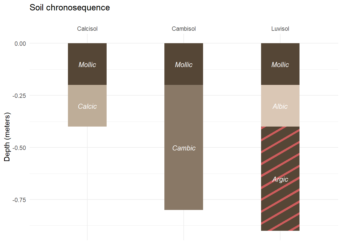
Finally, if we want to add single information on our plot, we may use annotate (instead of geom_).
soil_plot<-soil_plot+
  annotate(
    geom="segment",
    x=1,xend=3,
    y=-1,yend=-1,
    color="grey30",
    arrow=arrow()
  )+
  annotate(
    geom="text",
    x=2,y=-0.95,
    label="From 10,000s to 100,000s years",
    color="grey30",
    size=3.5, fontface="italic"
  )

soil_plot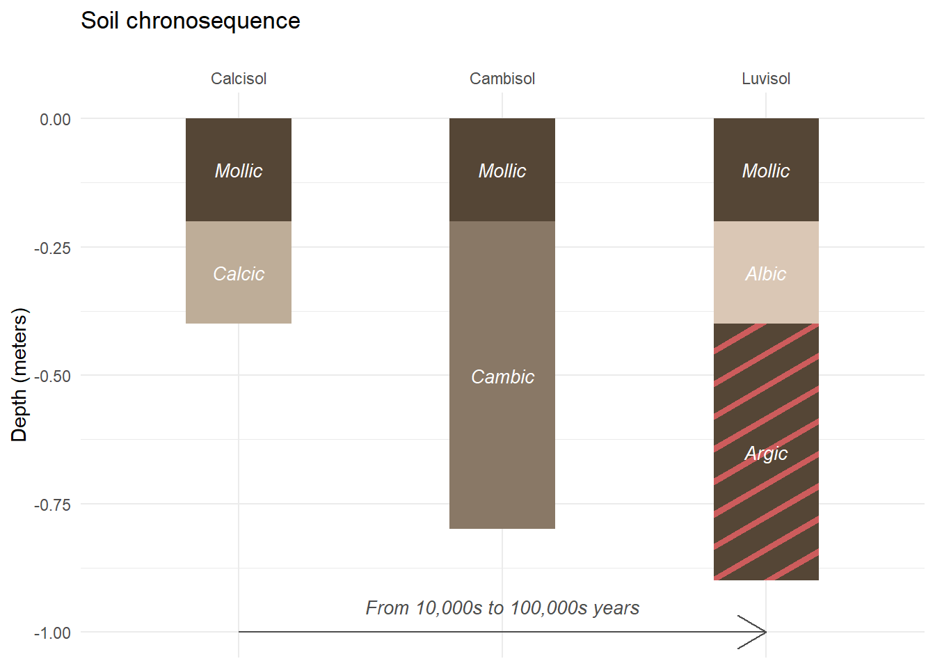
This framework should allow you to quickly start transforming your field observations into plots. Note that {ggpattern} has multiple options that you may use to plot other soil characteristics (coarse fragments, effervescence with hydrochloric acid…). Also, if you are interested in the representation of soil texture triangles, you may look at this post.
References
- Food and Agriculture Organization of the United Nations (FAO), 2014. World reference base for soil resources (WRB).
- Mike FC. ggpattern provides custom ggplot2 geoms which support filled areas with geometric and image-based patterns.
- Wickham C. Package ‘munsell’