Soil texture diagrams are widely used in agronomy but can be difficult to plot. Recently, Sara Acevedo published a flipbook showing how to plot soil texture diagrams with R. Following this example, let’s see how we can represent an important parameter related to soil texture: the water storage capacity.
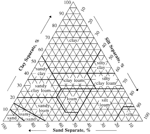
Figure 1 USDA soil textural triangle
Two packages are available to plot soil texture triangles with R: {soiltexture} specifically dedicated to soil texture triangles and {ggtern} for plotting all kind of ternary diagrams. Here we will use {ggtern} because of its compatibility with ggplot2.
1. Input creation
We will start by simulating a soil texture dataset with random values for clay, silt and sand content, while making sure that the sum of the three variables does not exceed 100%. To do so, we will use the RandVec() function from the {Surrogate} package.
library(tidyverse)
library(Surrogate)
library(magrittr)                # To change column name

N<-200                           # Setting number of draws

input<-RandVec(
  a=0, b=1,                    # Min/max values
  s=1,                         # Sum of all variables
  n=3,                           # Number of variables
  m=N                            # Number of draws
)

input<-t(input$RandVecOutput)%>%
  as.data.frame()%>%
  set_colnames(
    c("clay", "silt", "sand")    # Setting column names
  )

head(input)
## clay silt sand
## 1 0.10435077 0.6607402 0.2349090
## 2 0.04813742 0.6179598 0.3339027
## 3 0.08452404 0.7523101 0.1631658
## 4 0.28527675 0.2743642 0.4403590
## 5 0.01145161 0.1364547 0.8520937
## 6 0.44450927 0.4473236 0.1081672Next, we will use two pedotransfers function to estimate the two main soil water retention characteristics: the permanent wilting point (soil moisture content at which the plant will wilt and die) and field capacity (water content of the soil where all free water will drain form the soil through gravity). The water available to plants is between these two characteristic points
Here, we will use Rawls and Brakensiek (1985) equations to estimate the permanent wilting point and the field capacity. For simplicity, we will assume the same organic matter content for all samples.
input<-input%>%
  mutate(
    OM=0.025                                # OM content
  )%>%
  mutate(
    pwp=0.026+0.5*clay+1.58*OM              # Wilting point
  )%>%
  mutate(
    fc=0.2576-0.2*sand+0.36*clay+2.99*OM    # Field capacity
  )%>%
  mutate(
    uw_per=(fc-pwp)*100                     # "Usable" wetness
  )

head(input)
## clay silt sand OM pwp fc uw_per
## 1 0.10435077 0.6607402 0.2349090 0.025 0.11767538 0.3229345 20.525909
## 2 0.04813742 0.6179598 0.3339027 0.025 0.08956871 0.2828989 19.333021
## 3 0.08452404 0.7523101 0.1631658 0.025 0.10776202 0.3301455 22.238347
## 4 0.28527675 0.2743642 0.4403590 0.025 0.20813837 0.3469778 13.883945
## 5 0.01145161 0.1364547 0.8520937 0.025 0.07122580 0.1660538 9.482803
## 6 0.44450927 0.4473236 0.1081672 0.025 0.28775464 0.4707399 18.2985272. Plotting soil textures
Now, we can load {ggtern} to start plotting results.
library(ggtern)

textures<-ggtern(     # Specify ggtern instead of ggplot
  data=input,         # Same as {ggplot2}: specify data and aes()
  aes(
    x = sand,
    y = clay,
    z = silt
  )) +
  geom_point()

textures
Another way of using {ggtern} is to create a ‘regular’ {ggplot2} object, then add a third z dimension with coord_tern.
textures_ggplot<-ggplot(     # 'Regular' ggplot
  data=input,
  aes(
    x = sand,
    y = clay,
    z = silt
  )) +
  coord_tern(                # Add z coordinate to ggplot
    L='x',                   # Left pole
    T='y',                   # Top pole
    R='z'                    # Right pole
  )+
  geom_point()

textures_ggplot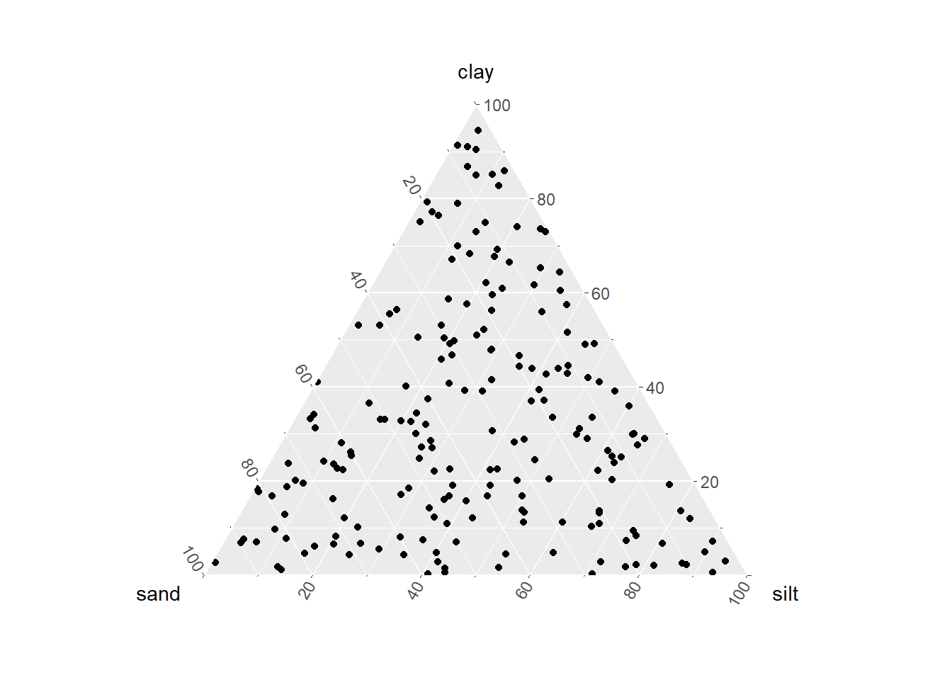
As you can see, {ggtern} shares the same syntax as {ggplot2}, which makes it easy to customize the plot with the same attributes as other plots. An important point is that we can use attributes like size and color according to a fourth variable
textures<-ggtern(
  data=input,aes(
    x = sand,
    y = clay,
    z = silt
  )) +
  geom_point(
    aes(color=uw_per),
    size=2,alpha=0.5
  )+
  scale_color_continuous(
    low="tomato",
    high="dodgerblue"
  )+
  labs(
    title="Diagram of available water",
    subtitle="Difference between field capacity and wilting point",
    color="Available water (%)"
  )+
  theme_bw()

textures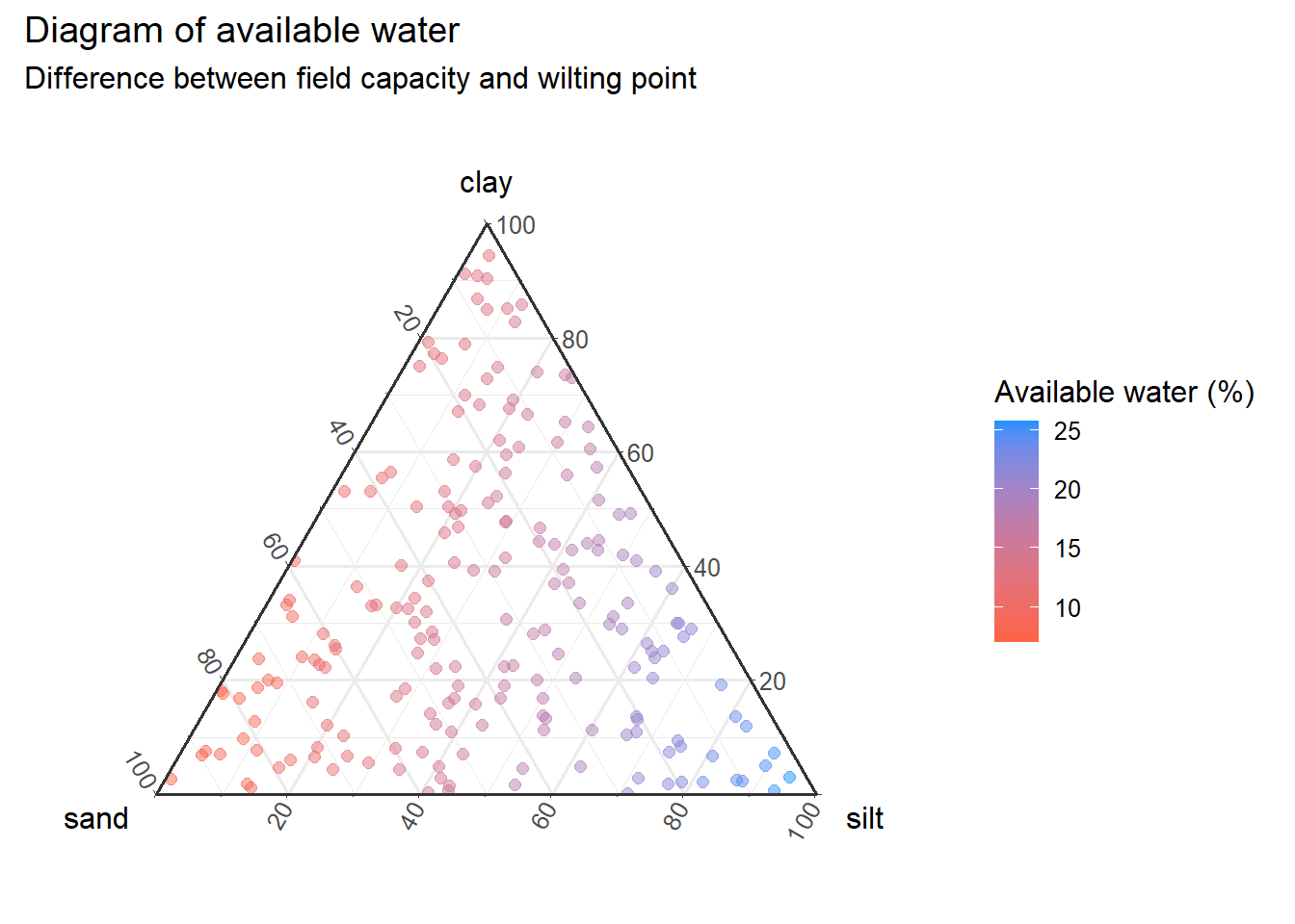
But {ggtern} also provides specific attributes for ternary diagrams.
textures_cust<-textures+
  geom_crosshair_tern(       # Highlight 1st sample
    data=head(input,1),
    lty="dashed",size=1,
    color="black"
  )+
  labs(
    yarrow = "Clay (%)",
    zarrow = "Silt (%)",
    xarrow = "Sand (%)"
  )+
  theme_showarrows()+        # Add arrows to axis titles
  theme_hidetitles()+
  theme_clockwise()          # Direction of ternary rotation

textures_cust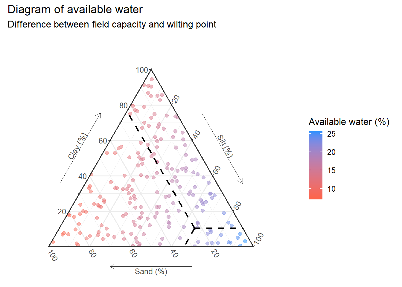
Now, if we want to plot the texture classes, {ggtern} contains the USDA texture triangle (but no other soil texture triangles).
data(USDA) # Load USDA
head(USDA)
## Clay Sand Silt Label
## 1 1.00 0.00 0.00 Clay
## 2 0.55 0.45 0.00 Clay
## 3 0.40 0.45 0.15 Clay
## 4 0.40 0.20 0.40 Clay
## 5 0.60 0.00 0.40 Clay
## 6 0.55 0.45 0.00 Sandy ClayWe can easily plot the classes boundaries with geom_polygon().
textures_classes<-textures_cust+
  geom_polygon(
    data=USDA,aes(x=Sand,y=Clay,z=Silt,group=Label),
    fill=NA,size = 0.3,alpha=0.5,
    color = "grey30"
  )

textures_classes
Plotting labels is a bit more complicated. Fortunately, Sara gave us a nice solution to prepare the labels before plotting:
USDA_text <- USDA  %>%
  group_by(Label) %>%
  summarise_if(is.numeric, mean, na.rm = TRUE) %>%
  ungroup()

head(USDA_text)
## # A tibble: 6 x 4
## Label Clay Sand Silt
## <fct> <dbl> <dbl> <dbl>
## 1 Clay 0.59 0.22 0.19
## 2 Sandy Clay 0.417 0.517 0.0667
## 3 Sandy Clay Loam 0.275 0.575 0.15
## 4 Sandy Loam 0.0929 0.621 0.286
## 5 Loamy Sand 0.0625 0.825 0.112
## 6 Sand 0.0333 0.917 0.05We can now add names with geom_text().
textures_names<-textures_classes+
  geom_text(
    data=USDA_text,
    aes(x=Sand,y=Clay,z=Silt,label=Label),
    size = 2,
    color = "grey30"
  )

textures_names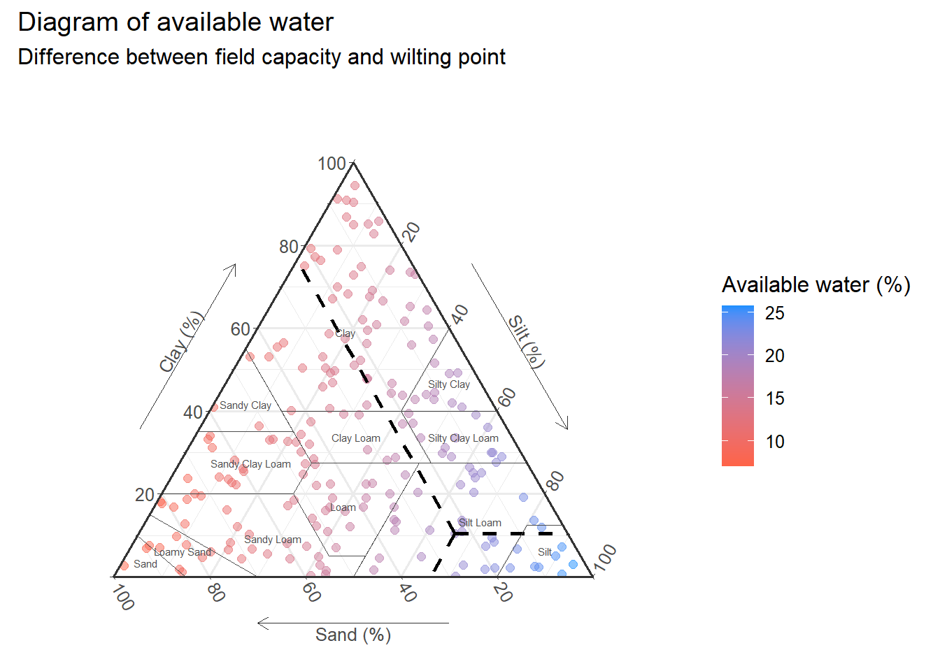
3. Data interpolation
Now that we have seen the main functions for representing data with {ggtern}, we will see how we can perform interpolations with the same package.
empty<-ggplot()+             # 'Regular' ggplot
  coord_tern(                # Add z coordinate to ggplot
    L='x',                   # Left pole
    T='y',                   # Top pole
    R='z'                    # Right pole
  )+
  labs(
    yarrow = "Clay (%)",
    zarrow = "Silt (%)",
    xarrow = "Sand (%)"
  )+
  theme_bw()+
  theme_showarrows()+        # Add arrows to axis titles
  theme_hidetitles()+
  theme_clockwise()          # Direction of ternary rotation

empty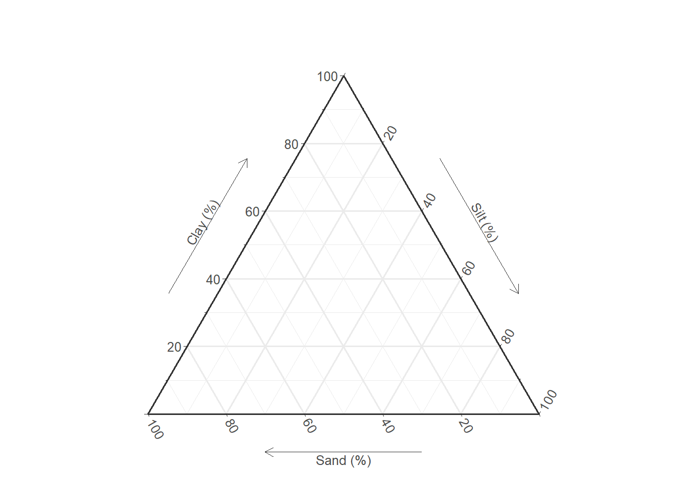
We will now add an interpolation of the available water based on the values of our input data set. To do so, we will use geom_interpolate_tern.
inter<-empty+
  geom_interpolate_tern(
    data=input,
    aes(
      x = sand,y = clay,z = silt,
      value = uw_per,
      color=..level..
    )
  )+scale_color_continuous(
    low="tomato",
    high="dodgerblue"
  )+
  labs(
    title="Diagram of available water",
    subtitle="Difference between field capacity and wilting point",
    color="Available water (%)"
  )
inter
As geom_smooth() in {ggplot2}, loess is the default smoothing method for {ggtern} (if the number of observations is less than 1000). We can also try different methods for interpolation. Below is an example with a linear model.
inter_lm<-empty+
  geom_interpolate_tern(
    data=input,
    aes(
      x = sand,y = clay,z = silt,
      value = uw_per,
      color=..level..
    ),
    method='lm',                      # Specify method
    formula=value~x+y,                # Specify formula
    n=100                             # Number of grid points
  )+scale_color_continuous(
    low="tomato",
    high="dodgerblue"
  )+
  labs(
    title="Diagram of available water",
    subtitle="Difference between field capacity and wilting point",
    color="Available water (%)"
  )
inter_lm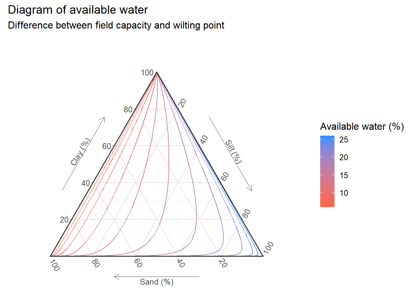
For a contour filled plot, we may use stat_interpolate_tern(). But this often requires tweaking the parameters to get the desired output.
fill_lm<-empty+
  stat_interpolate_tern(
    data=input,
    aes(
      x = sand,y = clay,z = silt,
      value = uw_per,
      fill=..level..
    ),
    geom="polygon",                  # add geom
    formula=value~x+y,
    method='lm',
    n=100,bins=100,                  # Increase for smoother result
    expand=1
  )+
  scale_fill_continuous(
    low="tomato",
    high="dodgerblue"
  )+
  labs(
    title="Diagram of available water",
    subtitle="Difference between field capacity and wilting point",
    fill="Available water (%)"
  )+
  geom_polygon(
    data=USDA,aes(x=Sand,y=Clay,z=Silt,group=Label),
    fill=NA,size = 0.3,alpha=0.5,
    color = "white"
  )+
  geom_text(
    data=USDA_text,
    aes(x=Sand,y=Clay,z=Silt,label=Label),
    size = 2,
    color = "white"
  )

fill_lm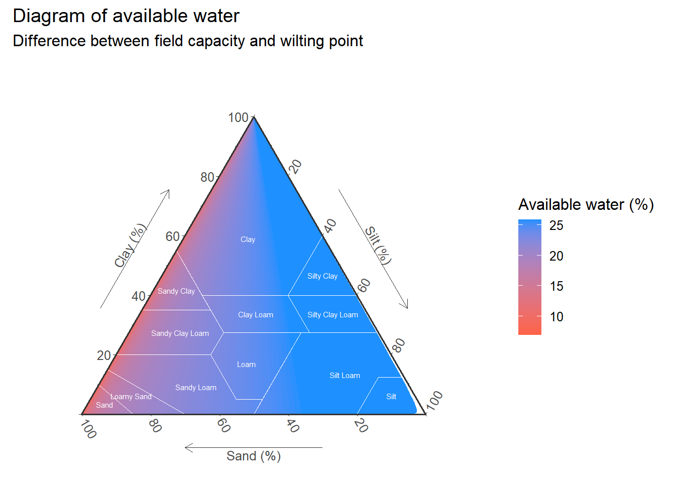
Acknowledgement
Many thanks to Sara Acevedo for sharing her presentation on soil texture triangles with R.
References
- Acevedo, S. (2021). Soil texture triangles using R.
- Hamilton, (2016). ggtern: ternary diagrams in R.
- Rawls, W. J. and Brakensiek D. L. (1985). Prediction of soil water properties for hydrologic modeling. Proceedings of Symposium on Watershed Management in the Eighties.