The tidyverse is a collection of extensions designed to work together and based on a common philosophy, making data manipulation and plotting easier. In this tutorial, we will use the tidyverse to program the first part of a crop model: the estimation of the number of plant leaves from temperature data, based on the work of Ringeval et al. (2021). This model will be applied to corn.
1. Model description
Before writing the model code, it is important to have defined the model structure.
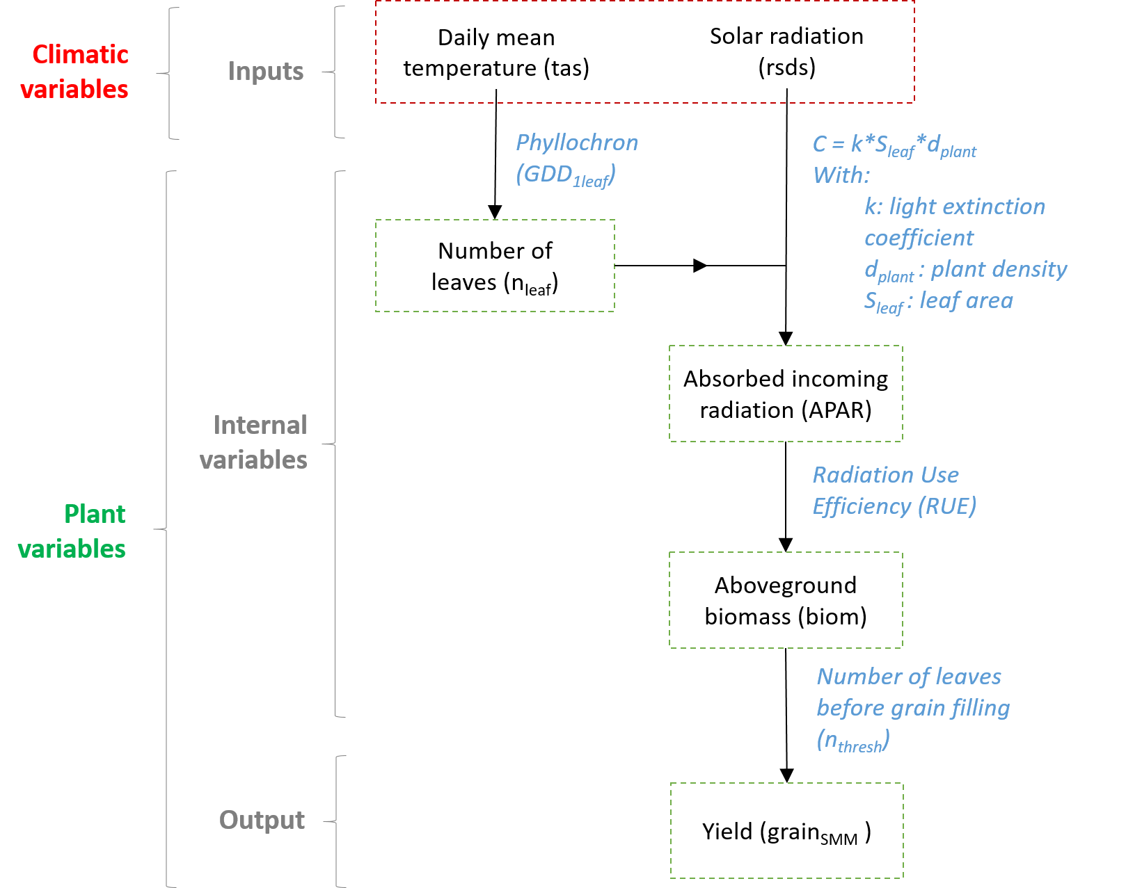
Figure 1 Model structure (adapted from Ringeval et al., 2021)
Briefly, this estimation of corn yield is done in three steps:
1. Estimation of number of leaves (based on daily temperature)
2. Estimation of the amount of photosynthetically active radiation intercepted by the plants
3. Conversion of this amount of radiation into biomass (first plant then grain)
We will now detail the equations related to the first part of the model: the estimation of the number of leaves
For any day, the thermal time (\(TT\), in °C) is computed from the daily mean temperature (\(tas\), in °C) by using a reference temperature under which plant growth stops (\(T_{0}\)): \[ \quad\text{(Eq. 1)}\quad \begin{cases} TT(day) = tas(day)-T_{0}, & tas(day)>T_{0} \\ 0 ,& tas(day)\leq T_{0} \end{cases} \]
Then, the sum of growing degree days (\(GDD\), in °C), may be defined as follows: \[ \quad\text{(Eq. 2)}\quad GDD(day)=\sum_{i} TT(i) \]
The number of leaves per plant (\(nleaf\)) is computed from GDD and two parameters: one representing the thermal requirement for the emergence of one leaf (\(GDD_{1leaf}\), in °C), the other the maximum number of leaves per plant (\(max_{nleaf}\)): \[ \quad\text{(Eq. 3)}\quad nleaf = min(max_{nleaf},\frac{GDD(day)}{GDD_{1leaf}}) \]
Hence, the model consists of one input variable (\(tas\)), two internal variables (\(TT\) and \(GDD\)), three parameters, (\(T_{0}\),\(GDD_{1leaf}\) and \(max_{nleaf}\)) and one output variable (\(nleaf\)).
2. Writing the model
2.1. Loading packages and inputs
The tidyverse is a collection of R packages designed for data science.

Figure 2 Core packages of the tidyverse (Barnier, 2021)
In this tutorial, we will mostly used {tidyr} and {dplyr} (for data handling) and {ggplot2} (for plotting).
The tidyverse may be loaded into R as follows:
# Install tidyverse (to do once)
# install.packages("tidyverse")
# Load tidyverse (to repeat at each session)
library(tidyverse)
As inputs, we will use one weather dataset from the National Centers for Environmental Information. For this tutorial, we will use weather data from Des Moines (USA). You may download the data required for this tutorial here. To be consistent with our model, we will use a daily time step data set. There are many weather variables in this dataset, but we will focus on the average daily temperature, which is the input required for our model.
# Load data
input <- read.table(file="Weather_DesMoines.csv", header=TRUE, sep=";",dec=".")
# Average daily temperature (in °C)
# (display only first values)
head(input$T_DAILY_MEAN)
## [1] 2.1 4.8 0.8 -2.8 2.2 0.32.2. Data preparation
For the rest of the tutorial, we will start from the input table and then progressively calculate the internal variables up to the output variable: the number of leaves. Thus, we will be close to the philosophy of the tidyverse.
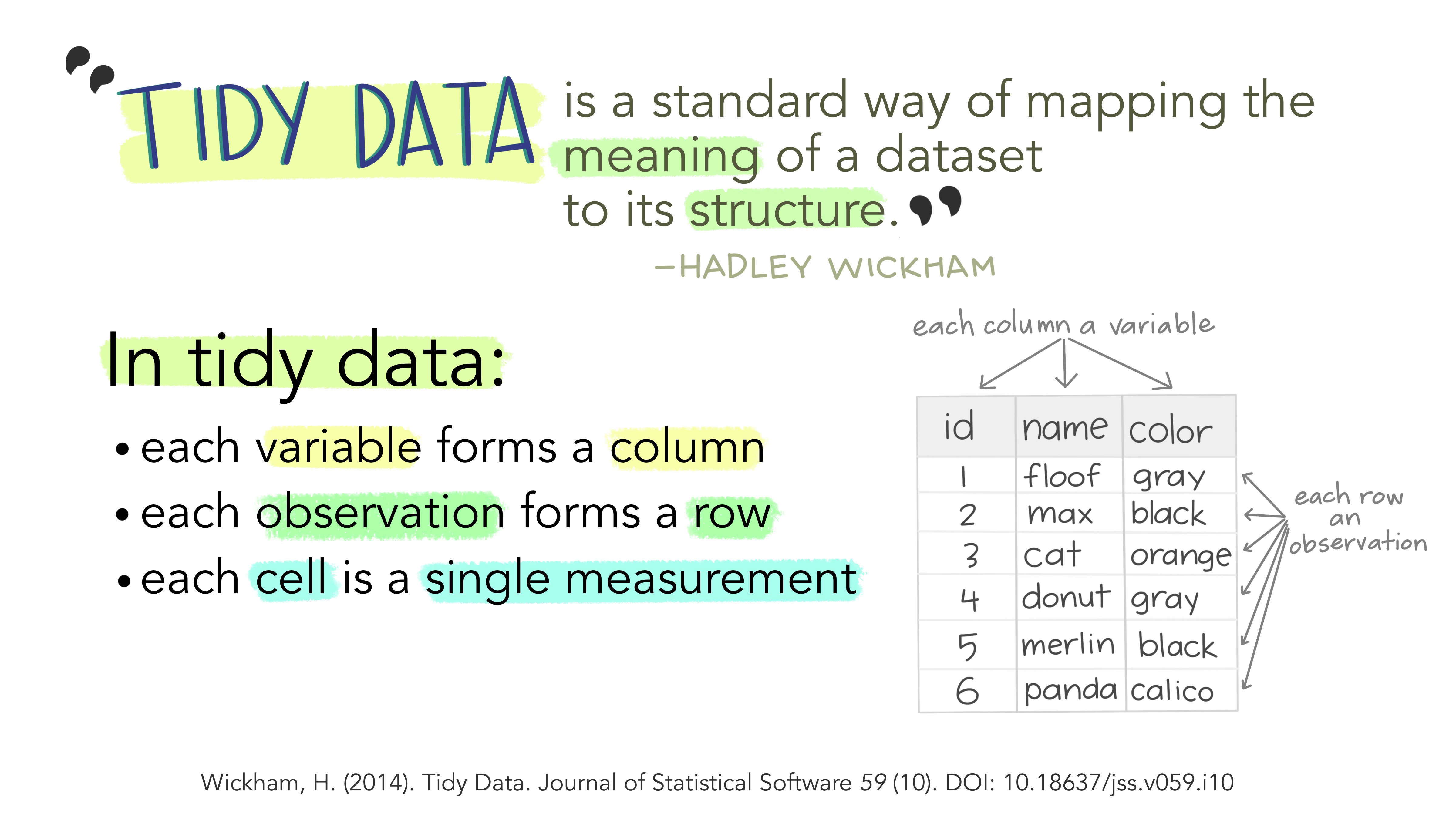
Figure 3 The “tidy” philosophy (Image credit: Allison Horst)
To do so, we will use a combination of functions assembled thanks to the pipe operator (%>%), which allows to perform a sequence of actions.
As a first step, using the select() function from the {dplyr} package, we will select only the column with daily mean temperature and solar radiation, which are the only climate variables used in the model. In this step, we will also rename the variables in the same way as in the model, for more clarity.
# Creating 'data' from 'input':
# select only mean T° data
data<-input%>%                  # Best practice: line break after %>%,
  dplyr::select(                # then each new line indented by two spaces
    tas = T_DAILY_MEAN,
    rsds = SOLARAD_DAILY        # New name = Old name
  )
head(data)
## tas rsds
## 1 2.1 6.81
## 2 4.8 7.23
## 3 0.8 1.49
## 4 -2.8 3.17
## 5 2.2 7.75
## 6 0.3 5.87Then, to add new columns, we will mainly use the mutate() function, also from {dplyr}.
We will now use mutate() to add day number to our input table. As the table is ordered chronologically from January 1st to December 31st, we are going to create this new column thanks to the number of the rows that can be obtained with the row_number() function.
data<-input%>%
  dplyr::select(
    tas = T_DAILY_MEAN,
    rsds = SOLARAD_DAILY
  )%>%
  dplyr::mutate(
    day_number = row_number()     # Add a new column with day number
  )

head(data)
## tas rsds day_number
## 1 2.1 6.81 1
## 2 4.8 7.23 2
## 3 0.8 1.49 3
## 4 -2.8 3.17 4
## 5 2.2 7.75 5
## 6 0.3 5.87 6In this tutorial, we are interested in corn development. Therefore, we will keep only dates between standard sowing and harvest dates for the area. To do so, we will use the filter() function.
day_sowing<-92                       # Sowing after 1st May
day_harvest<-287                     # Harvest ~ mid-october

data<-input%>%
  dplyr::select(
    tas = T_DAILY_MEAN,
    rsds = SOLARAD_DAILY
  )%>%
  dplyr::mutate(
    day_number = row_number()
  )%>%
  dplyr::filter(
    day_number>=day_sowing,
    day_number<=day_harvest
  )

head(data)
## tas rsds day_number
## 1 9.7 19.37 92
## 2 13.6 10.18 93
## 3 4.3 1.72 94
## 4 3.1 18.13 95
## 5 7.7 22.15 96
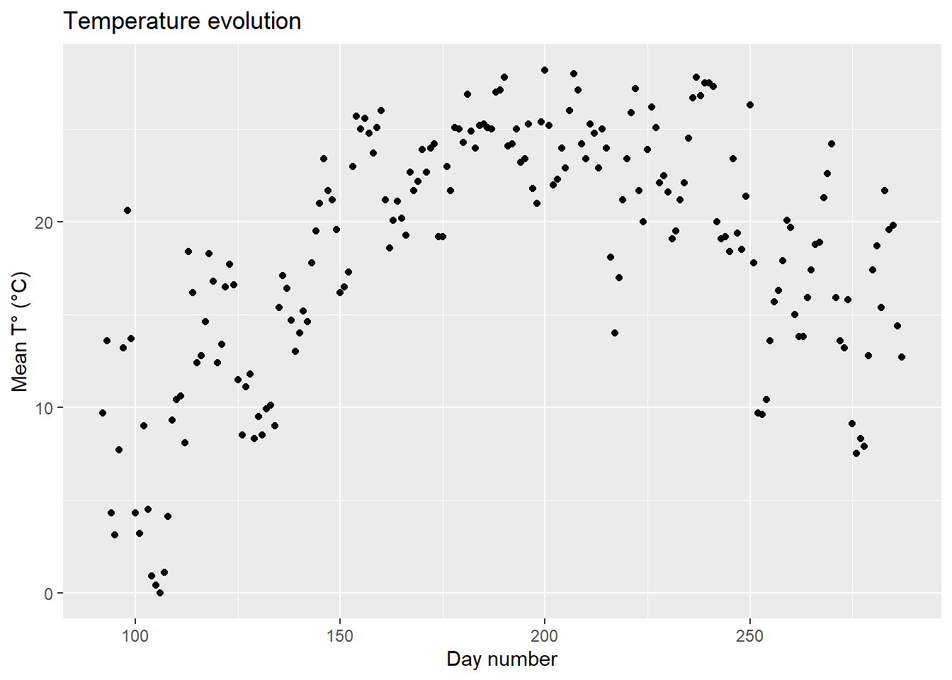
## 6 13.2 4.78 97Now we can already make a first representation of the data with {ggplot2}: the evolution of the temperatures during the growing season. The basic principle of {ggplot2} is that we will first specify the data we want to use within the ggplot() function, then specify the layers we want to add with the + operator.
ggplot2::ggplot(
    data=data,                           # Name of the data frame to be used
    aes(x=day_number, y=tas)             # Specify x and y axis
  )+
  geom_point()+                          # Add points to the plot
  labs(                                  # Customize labels
    title = "Temperature evolution",
    x = "Day number",
    y = "Mean T° (°C)"
  )
Like geom_point(), there are many geom layers that can be added to ggplot(). before we start programming our model, we will just see how we can add a smoothing layer with geom_smooth() (note that there are many ways to customize graphs with {ggplot2}, but that we will not go into details in this tutorial).
ggplot2::ggplot(
    data=data,
    aes(x=day_number, y=tas)
  )+
  geom_point(color="darkslategray3")+      # Change color of geom_point()
  geom_smooth(color="darkslategray")+      # Add smoothing layer
  labs(
    title = "Temperature evolution",
    x = "Day number",
    y = "Mean T° (°C)"
  )
## `geom_smooth()` using method = 'loess' and formula 'y ~ x'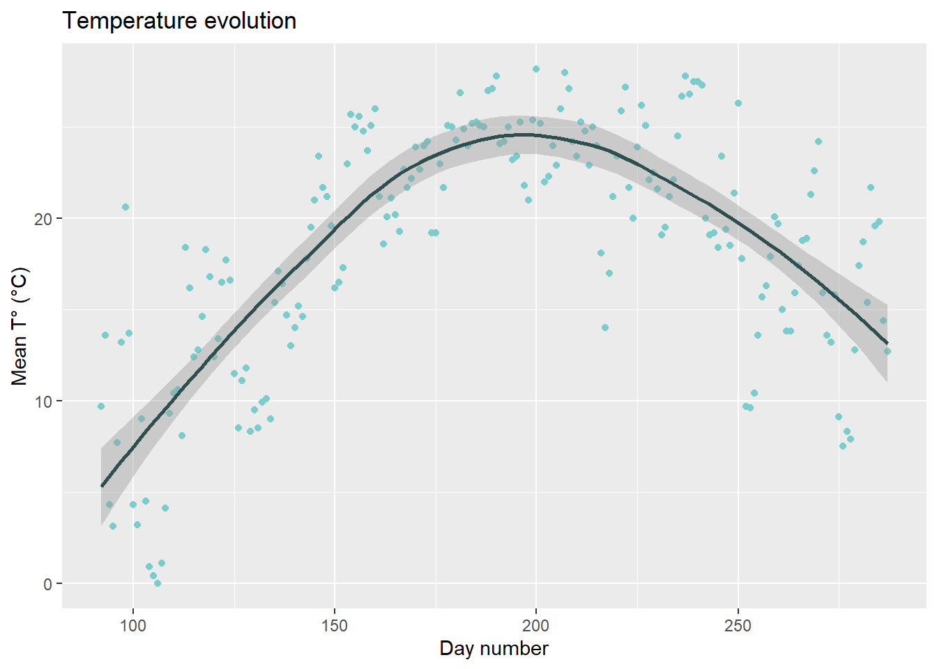
2.3. Writing model equations
To simplify the following explanations, we will write the model from the data table created above, but it should be noted that it would be possible to pursue the chain of actions started from the input table.
The mutate() function will again be used to calculate \((Eq. 1)\) and add thermal time (\(TT\)) to data table. However, this case is a little bit different because there is a condition (daily temperature above or below \(T_{0}\)). This condition may be expressed with the case_when() function.
T0<-6 # Set T0 for corn: 6°C

model<-data%>%
  dplyr::mutate(
    TT=dplyr::case_when(
      tas<T0~0,                 # Condition 1 ~ Column value
      tas>=T0~tas-T0            # Condition 2 ~ Volumn value
    )
  )
# Print first rows
head(model)
## tas rsds day_number TT
## 1 9.7 19.37 92 3.7
## 2 13.6 10.18 93 7.6
## 3 4.3 1.72 94 0.0
## 4 3.1 18.13 95 0.0
## 5 7.7 22.15 96 1.7
## 6 13.2 4.78 97 7.2We may then calculate growing degree days (\(GDD\)) from \((Eq. 2)\) using the cumsum() function available in base R.
model<-data%>%
  dplyr::mutate(
    TT=dplyr::case_when(
      tas<T0~0,
      tas>=T0~tas-T0
    )
  )%>%
  mutate(
    GDD = cumsum(TT)                   # Cumulative sum of thermal time
  )
# Print last rows
tail(model)
## tas rsds day_number TT GDD
## 191 15.4 15.51 282 9.4 2417.8
## 192 21.7 14.71 283 15.7 2433.5
## 193 19.6 15.08 284 13.6 2447.1
## 194 19.8 14.57 285 13.8 2460.9
## 195 14.4 16.28 286 8.4 2469.3
## 196 12.7 15.98 287 6.7 2476.0Finally, to estimate the number of leaves, we will split \((Eq. 1)\) into two parts: estimation of the potential number of leaves, then comparison with the maximum possible number of leaves per plant.
# Set parameters:
# Sum of T° for the emergence of 1 leaf
GDD_1leaf<-50
# Maximum number of leaves per plant
max_nleaf<-20

model<-data%>%
  dplyr::mutate(
    TT=dplyr::case_when(
      tas<T0~0,
      tas>=T0~tas-T0
    )
  )%>%
  mutate(
    GDD = cumsum(TT)
  )%>%
  # Potential number of leaves (no max values)
  mutate(
    pot_nleaf = GDD/GDD_1leaf
  )%>%
  # Estimated number of leaves (including max)
  mutate(
    nleaf = case_when(
      pot_nleaf<=max_nleaf~round(pot_nleaf),
      pot_nleaf>max_nleaf~max_nleaf
    )
  )

tail(model)
## tas rsds day_number TT GDD pot_nleaf nleaf
## 191 15.4 15.51 282 9.4 2417.8 48.356 20
## 192 21.7 14.71 283 15.7 2433.5 48.670 20
## 193 19.6 15.08 284 13.6 2447.1 48.942 20
## 194 19.8 14.57 285 13.8 2460.9 49.218 20
## 195 14.4 16.28 286 8.4 2469.3 49.386 20
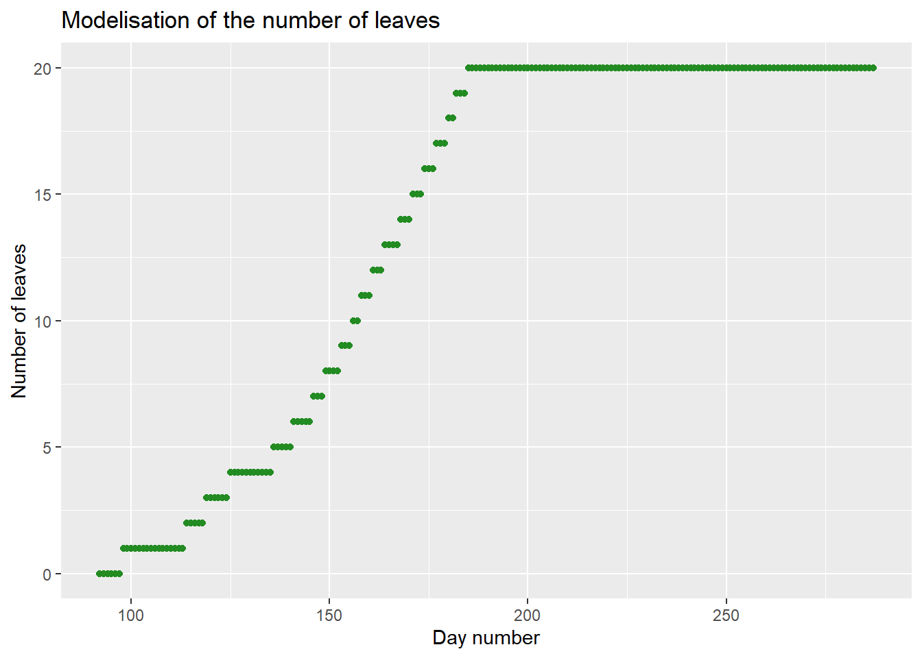
## 196 12.7 15.98 287 6.7 2476.0 49.520 20Results may also be represented with {ggplot2}.
ggplot2::ggplot(
    data=model,
    aes(x=day_number, y=nleaf)
  )+
  geom_point(color="forestgreen")+
  labs(
    title = "Modelisation of the number of leaves",
    x = "Day number",
    y = "Number of leaves"
  )
3. Using the model
3.1. Creating a function
In order to facilitate the realization of multiple simulations, it is appropriate to transform the code defined above into a function. The creation of a function follows the structure below:
function_name <- function(arguments) {
    instructions
    return(results)
}
For example, we will create a function with three agruments that will allow us to evaluate the effect of the thermal requirement for the emergence of one leaf (\(GDD_{1leaf}\), also called phyllochron) on the evolution of the number of leaves.
model_fun <- function(
  name,           # Scenario name
  data,           # Climatic variables to be used as inputs
  GDD_1leaf       # Thermal requirement for the emergence of one leaf
  ){

  # Set parameters (without GDD_1leaf)
  max_nleaf<-20
  T0<-6
  # Estimate nleaf
  model<-data%>%
    dplyr::mutate(
      TT=dplyr::case_when(
        tas<T0~0,
        tas>=T0~tas-T0
    ))%>%
    mutate(
      GDD = cumsum(TT)
    )%>%
    mutate(
      pot_nleaf = GDD/GDD_1leaf
    )%>%
    mutate(
      nleaf = case_when(
        pot_nleaf<=max_nleaf~round(pot_nleaf),
        pot_nleaf>max_nleaf~max_nleaf
      )
    )%>%
    add_column(                                # To add scenario name to data
      Scenario = name                          # (set 'name' in argument)
    )
  return(model)
}

# Test the function for baseline scenario
baseline <- model_fun(name="Baseline",data=data,GDD_1leaf = 40)
tail(baseline)
## tas rsds day_number TT GDD pot_nleaf nleaf Scenario
## 191 15.4 15.51 282 9.4 2417.8 60.4450 20 Baseline
## 192 21.7 14.71 283 15.7 2433.5 60.8375 20 Baseline
## 193 19.6 15.08 284 13.6 2447.1 61.1775 20 Baseline
## 194 19.8 14.57 285 13.8 2460.9 61.5225 20 Baseline
## 195 14.4 16.28 286 8.4 2469.3 61.7325 20 Baseline
## 196 12.7 15.98 287 6.7 2476.0 61.9000 20 BaselineWe can now use this function to evaluate the effect of \(GDD_{1leaf}\), assuming, for example, that we can reduce this parameter through plant breeding.
baseline <- model_fun(
  name="Baseline", data=data, GDD_1leaf = 50
)
breed <- model_fun(
  name="Improved cultivar",data=data, GDD_1leaf = 40
)

comp<-rbind.data.frame(                         # Merging results
  baseline,                                     # before plotting
  breed
)

ggplot(
    data=comp,
    aes(x=day_number,y=nleaf,color=Scenario)    # Add color in aes()
  )+
  geom_point()+
    labs(
    title = "Comparison between two cultivars",
    x = "Day number",
    y = "Number of leaves"
  )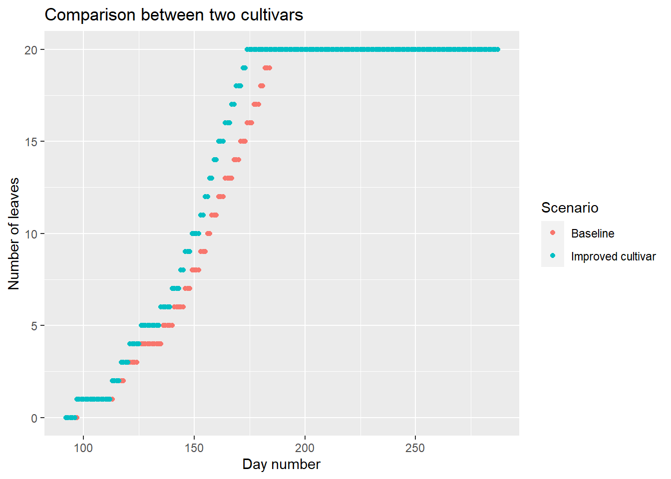
Following this example, the function can be used to compare many scenarios.
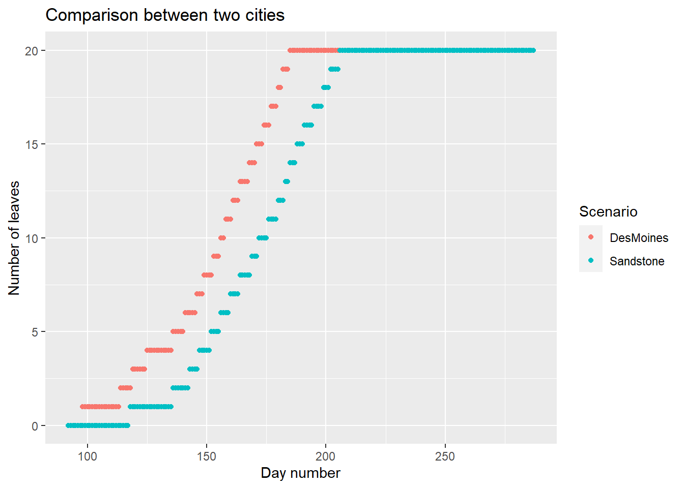
Application Use the model to compare the number of leaves between two cities: DesMoines (Iowa) and Sandstone (Minnesota)
# Load second datafile
input_sandstone <- read.table(file="Weather_Sandstone.csv", header=TRUE, sep=";",dec=".")
# Cleaning data
data_sandstone<-input_sandstone%>%
  dplyr::select(
    tas = T_DAILY_MEAN,
    rsds = SOLARAD_DAILY
  )%>%
  dplyr::mutate(
    day_number = row_number()
  )%>%
  dplyr::filter(
    day_number>=day_sowing,
    day_number<=day_harvest
  )
# Apply function for both datasets
baseline <- model_fun(
  name="DesMoines", data=data, GDD_1leaf = 50
)
sandstone <- model_fun(
  name="Sandstone",data=data_sandstone, GDD_1leaf = 50
)
# Merging results before plotting
comp<-rbind.data.frame(
  baseline,
  sandstone
)
# Plotting
ggplot(
    data=comp,
    aes(x=day_number,y=nleaf,color=Scenario)
  )+
  geom_point()+
    labs(
      title = "Comparison between two cities",
      x = "Day number",
      y = "Number of leaves"
  )
3.2. Going further
Following this tutorial, you may now complete the function based on the equations given by Ringeval et al. (2021) to obtain a model for estimating yield from weather data (a suggestion is given in the Appendix). In the second part, we will see how to analyze the performance of this model (sensitivity analysis and uncertainty analysis).
Acknowledgement
Many thanks to Bruno Ringeval for taking the time to answer my questions.
References
- Barnier, J. (2021). Introduction à R et au tidyverse. https://juba.github.io/tidyverse/index.html
- Ringeval, B. et al. (2021). Potential yield simulated by global gridded crop models: using a process-based emulator to explain their differences. Geosci. Model Dev., 14, 1639–1656. https://doi.org/10.5194/gmd-14-1639-2021
Appendix
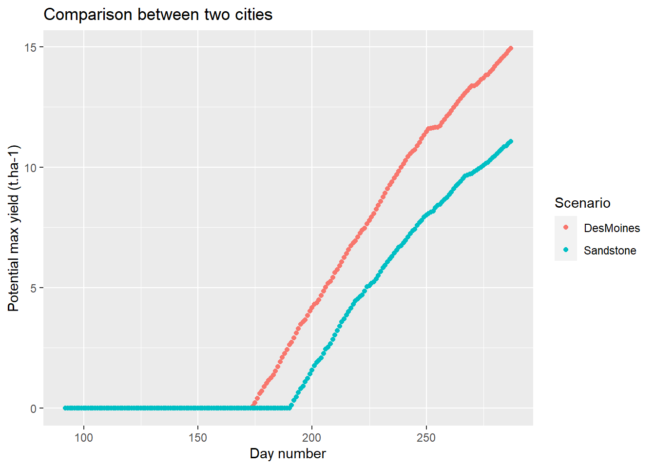
You will find below a suggestion to code the whole model and estimate potential maximum corn yield from temperature and solar radiation.
# Outside the function:
# Required parameters to compute C
# Light extinction coefficient
K <- 0.56
# Individual leaf area (m-2)
S <- 0.05
# Plant density (m-2)
d <- 90000/10000

# Model function
model_fun <- function(
  name,           # Scenario name
  data,           # Climatic variables to be used as inputs
  GDD_1leaf,      # Thermal requirement for the emergence of one leaf
  C,              # C=f(K,S,d)
  RUE,            # Radiation use efficiency (gDM.MJ-1)
  nthresh         # Number of leaves before grain filling
  ){
  # Set parameters (without GDD_1leaf)
  max_nleaf<-20
  T0<-6
  f<-0.5      # Active fraction of incoming radiation
  frac<-0.7   # Fraction of Net Primary Productivity dedicated to grain

  # Estimate yield
  model<-data%>%
    dplyr::mutate(
      TT=dplyr::case_when(
        tas<T0~0,
        tas>=T0~tas-T0
    ))%>%
    mutate(
      GDD = cumsum(TT)
    )%>%
    mutate(
      pot_nleaf = GDD/GDD_1leaf
    )%>%
    mutate(
      nleaf = case_when(
        pot_nleaf<=max_nleaf~round(pot_nleaf),
        pot_nleaf>max_nleaf~max_nleaf
      )
    )%>%
     # Incoming photosynthetic active radiation (MJ.m-2.day-1)
    mutate(
      PAR_inc = f*rsds
    )%>%
    # Absorbed PAR by the canopy (MJ.m-2.day-1)
    mutate(
      APAR = PAR_inc*(1-exp(-C*nleaf))
    )%>%
    # Net primary productivity dedicated to the aboveground biomass
    mutate(
      NPP = RUE*APAR
    )%>%
    # Sum of aboveground biomass
    mutate(
      biom = cumsum(NPP)
    )%>%
    # Net primary productivity dedicated to the variable grain
    mutate(
      NPPgrain = case_when(
        nleaf<nthresh ~ 0,
        nleaf>=nthresh ~ frac*NPP
      )
    )%>%
    # Total grain production (g.m-2)
    mutate(
      grain = cumsum(NPPgrain)
    )%>%
    # Total grain production (t.ha-1)
    mutate(
      grain_t = grain/100
    )%>%
    add_column(                                # To add scenario name to data
      Scenario = name                          # (set 'name' in argument)
    )
  return(model)
}


# Apply function for both datasets
baseline <- model_fun(
  name="DesMoines",
  data=data,
  GDD_1leaf = 50,
  C=K*S*d,
  RUE=2,
  nthresh = 16
)
sandstone <- model_fun(
  name="Sandstone",
  data=data_sandstone,
  GDD_1leaf = 50,
  C=K*S*d,
  RUE=2,
  nthresh = 16
)
# Merging results before plotting
comp<-rbind.data.frame(
  baseline,
  sandstone
)
# Plotting
ggplot(
    data=comp,
    aes(x=day_number,y=grain_t,color=Scenario)
  )+
  geom_point()+
  labs(
    title = "Comparison between two cities",
    x = "Day number",
    y = "Potential max yield (t.ha-1)"
  )