In the first part) of this tutorial, we created the model. In the second part we analyzed the uncertainty associated with the model predictions. We will now evaluate the error associated with the model predictions (the Root Mean Square Error, RMSE), and then try to decrease this error by optimizing the \(RUE\) parameter, which we previously identified as the one that most influenced the model results.
1. Simulate multiple scenarios
First step is to apply our model to multiple situations simultaneously. We will focus on a geographical area that roughly covers the state of Iowa, in which the city of DesMoines that we studied earlier is located.
1.1. Prepare the data
Weather data in the file Weather_Iowa.csv (available here). Units of temperature and radiation measurements must be changed before they are used in the model:
# Load tidyverse
library(tidyverse)
# Load data
input <- read.table(file="Weather_Iowa.csv", header=TRUE, sep=",",dec=".")

day_sowing<-92                       # Sowing after 1st May
day_harvest<-287                     # Harvest ~ mid-october

data<-input%>%
  dplyr::filter(
    day_number>=day_sowing,
    day_number<=day_harvest
  )%>%
  mutate(
    tas=tas-273,15                   # Convert kelvin to degrees
  )%>%
  mutate(
    rsds=rsds*10^(-6)*24*60*60       # Convert watt to MJ.day-1
  )

head(data)
## X Coordinates lon lat day_number tas rsds 15
## 1 3 -91.25_40.25 -91.25 40.25 100 8.750000 24.450177 15
## 2 4 -91.25_40.25 -91.25 40.25 101 8.375000 8.501291 15
## 3 5 -91.25_40.25 -91.25 40.25 102 6.125000 9.225413 15
## 4 6 -91.25_40.25 -91.25 40.25 103 6.299988 23.274854 15
## 5 7 -91.25_40.25 -91.25 40.25 104 9.875000 24.700177 15
## 6 8 -91.25_40.25 -91.25 40.25 105 14.750000 25.525130 15Another important step in the preparation of the data will be to set the variable “Coordinates” as a factor. In the following steps, this will allow us to apply the model to each grid cell
data<-data%>%
  select(
    Coordinates, lon, lat,                 # Only keep requested variables
    day_number, tas, rsds
  )%>%
  mutate(
    Coordinates=as.factor(Coordinates)     # Set column coordinates as factor
  )
head(data)
## Coordinates lon lat day_number tas rsds
## 1 -91.25_40.25 -91.25 40.25 100 8.750000 24.450177
## 2 -91.25_40.25 -91.25 40.25 101 8.375000 8.501291
## 3 -91.25_40.25 -91.25 40.25 102 6.125000 9.225413
## 4 -91.25_40.25 -91.25 40.25 103 6.299988 23.274854
## 5 -91.25_40.25 -91.25 40.25 104 9.875000 24.700177
## 6 -91.25_40.25 -91.25 40.25 105 14.750000 25.525130Before applying the model, we can map our study area.
theme_custom<-theme(
    panel.background = element_blank()     # Hide grey filling behind plot
)

map<-ggplot(data=data,aes(x=lon,y=lat))+
  labs(
    title="Coordinates for the dataset",
    subtitle="Projection: WGS84",
    x="Longitude",
    y="Latitude"
  )+
  theme_custom

map+
  geom_tile(color="grey",fill="white")     # Plot grid on the map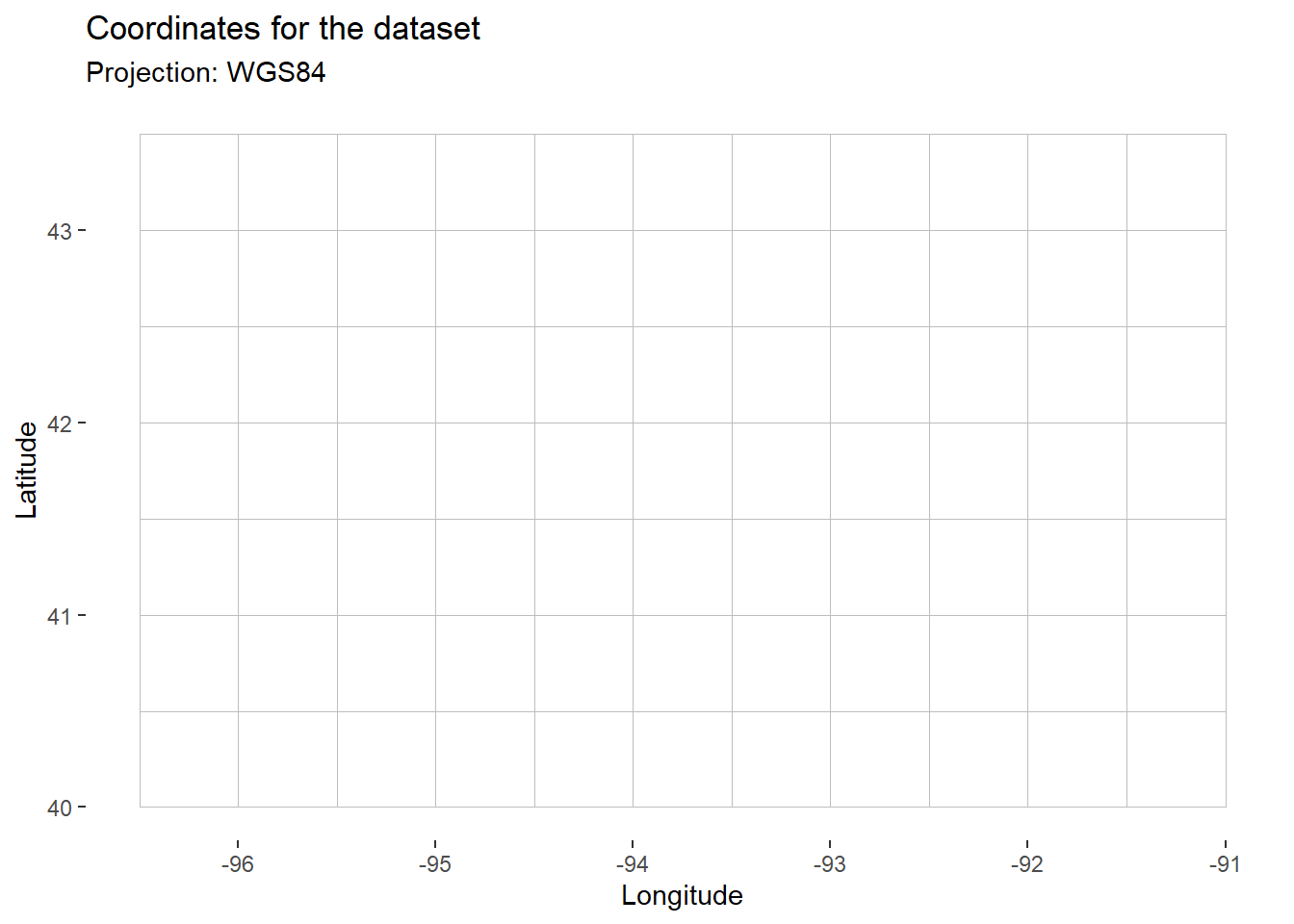
We have eleven units in longitude and seven in latitude, that is 77 cells on which we will apply the model.
For this study area, we can also map daily temperature or solar radiation. Below is an example of daily temperature at sowing date.
map_temp<-map+
  geom_tile(
    data=filter(data,day_number==day_sowing),   # Keep only data for sowing date
    aes(x=lon,y=lat,fill=tas)                   # Fill with temperature
  )+
  labs(
    fill="Temp. (°C)"
  )
map_temp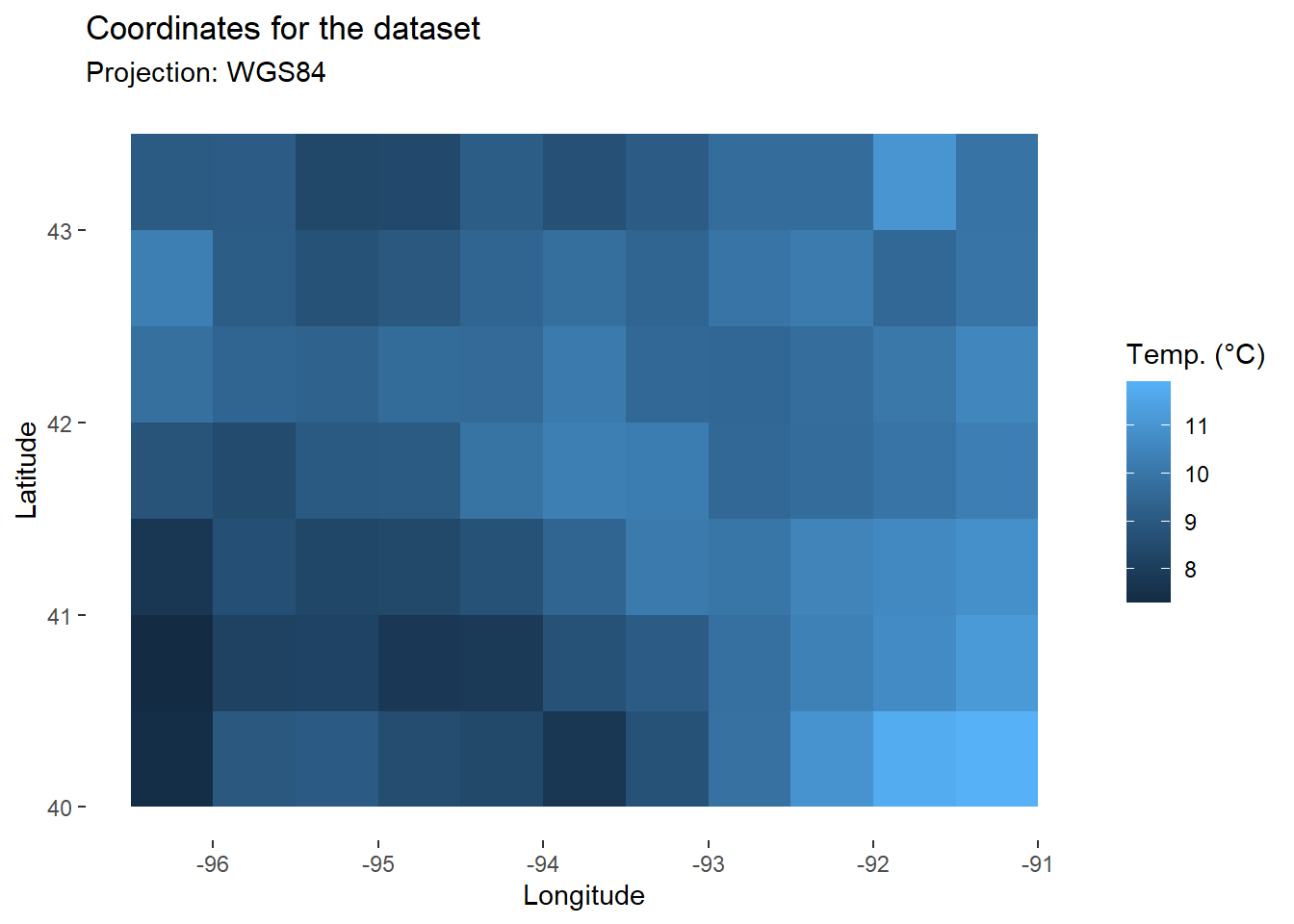
Finally, we will use annotate() to add to the map the city of DesMoines, which we have studied in the first two parts of the tutorial (longitude: -93.615451, latitude: 41.570438).
DM_loc<-annotate(
    geom="point",                         # Add one point for DesMoines
    x=-93.615451, y=41.570438,
    color="white"
  )
DM_name<-annotate(                        # Add city name as label
    geom="text",
    x=-93.615451, y=41.570438+0.2,        # (slight shifts not to overlap the city name)
    label="Des Moines",
    color="white"
  )

map_temp+
  DM_loc+
  DM_name
1.2. Apply model
As shown above, our input table has data for 77 different situations. We cannot therefore use exactly the same function as in the first two parts of the tutorial. We need to modify our fonction to include group_by(), a function from {dplyr} that will convert our input table into a grouped table where operations are performed “by group”.

Figure 1 group_by() and ungroup() (Image credit: Allison Horst)
To illustrate this, we will apply group_by() to the very first step of our model: the computation of the sum of Growing Degree Days (\(GDD\)). To perform this sum for each cell of the map (and not for all 77 cells), we will use the “Coordinates” factor.
T0<-6                                          # Set base T° for corn

model<-data%>%
  dplyr::mutate(
    TT=dplyr::case_when(
      tas<T0~0,
      tas>=T0~tas-T0
  ))%>%
  group_by(Coordinates)%>%                   # Specify grouping factor
  arrange(day_number,by_group=TRUE)%>%       # Order by day_number
  mutate(
    GDD = cumsum(TT)
  )%>%
  ungroup()                                  # End grouping

# Number of rows for input/output ?
rbind(
  nrow(data),
  nrow(model)
)
## [,1]
## [1,] 15092
## [2,] 15092Grouping does not change how the data looks (here data and model tables have the same number of rows), it changes how it interacts with other functions. We can see this when mapping the sum of Growing Degree Days: a specific \(GDD\) was calculated for each cell.
map_gdd<-ggplot(
  data=filter(model,day_number==day_harvest),
  aes(x=lon,y=lat))+
  geom_tile(aes(fill=GDD))+                     # Fill tile according to GDD
  labs(
    title="Mapping Growing Degree Days",
    subtitle="Projection: WGS84",
    x="Longitude",
    y="Latitude",
    fill="GDD (°C)"
  )+
  theme_custom

map_gdd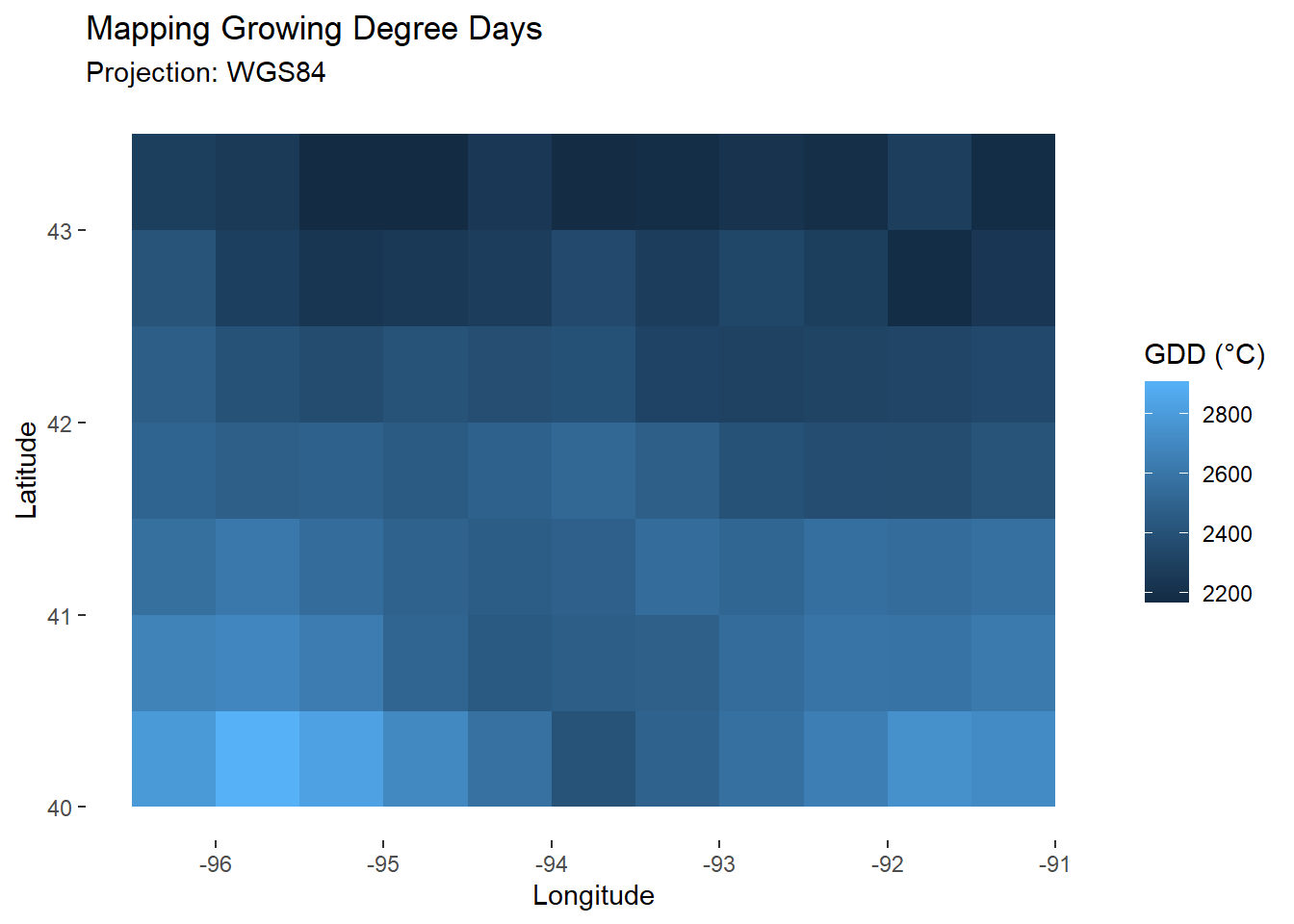
As in the example above, we will now include group_by() in the function used in the first two parts of the tutorial. This will allow us to estimate the final yield for each cell in our study area.
Also, in order to simplify the function, we will only keep data (for the input table) and \(C\) and \(RUE\) as arguments, and move the other parameters inside the function.
# Model function
model_whole_fun <- function(data,C,RUE){

  # Set parameters
  GDD_1leaf<-50   # Thermal requirement for the emergence of one leaf
  max_nleaf<-20   # Max number of leaves
  nthresh<-16     # Number of leaves before grain filling
  T0<-6           # Base temperature for corn
  f<-0.5          # Active fraction of incoming radiation
  frac<-0.7       # Fraction of Net Primary Productivity dedicated to grain

  # Estimate yield
  model<-data%>%
    dplyr::mutate(
      TT=dplyr::case_when(
        tas<T0~0,
        tas>=T0~tas-T0
    ))%>%
    group_by(Coordinates)%>%              # TO INCLUDE: grouping by Coordinates
    arrange(day_number,by_group=TRUE)%>%  # + arrange by day_number
    mutate(
      GDD = cumsum(TT)
    )%>%
    mutate(
      pot_nleaf = GDD/GDD_1leaf
    )%>%
    mutate(
      nleaf = case_when(
        pot_nleaf<=max_nleaf~round(pot_nleaf),
        pot_nleaf>max_nleaf~max_nleaf
      )
    )%>%
    # Incoming photosynthetic active radiation (MJ.m-2.day-1)
    mutate(
      PAR_inc = f*rsds
    )%>%
    # Absorbed PAR by the canopy (MJ.m-2.day-1)
    mutate(
      APAR = PAR_inc*(1-exp(-C*nleaf))
    )%>%
    # Net primary productivity dedicated to the aboveground biomass
    mutate(
      NPP = RUE*APAR
    )%>%
    # Sum of aboveground biomass
    mutate(
      biom = cumsum(NPP)
    )%>%
    # Net primary productivity dedicated to the variable grain
    mutate(
      NPPgrain = case_when(
        nleaf<nthresh ~ 0,
        nleaf>=nthresh ~ frac*NPP
      )
    )%>%
    # Total grain production (g.m-2)
    mutate(
      grain = cumsum(NPPgrain)
    )%>%
    # Total grain production (t.ha-1)
    mutate(
      grain_t = grain/100
    )%>%
    ungroup()                             # TO INCLUDE: End grouping

  return(model)

}
We can now apply our model to the whole study area.
model <- model_whole_fun(data=data, C=0.2, RUE=2)   # Apply function

map_yield<-ggplot(
  data=filter(model,day_number==day_harvest),       # Keep only final values
  aes(x=lon,y=lat,fill=grain_t))+                   # Fill according to final yield
  geom_tile()+                                      # Add tiles
  labs(
    title="Final yield",
    subtitle="Projection: WGS84",
    x="Longitude",
    y="Latitude",
    fill="Yield (t.ha-1)"                           # Specify fill legend
  )+
  theme_custom

map_yield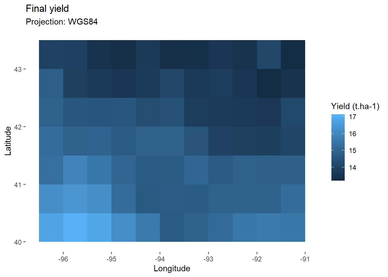
If you like, you can choose a more classic color scale for tile filling.
map_yield+
  scale_fill_gradient(
    low="red",            # Set color for low values
    high="green"          # Set color for high values
  )+
  DM_loc+
  DM_name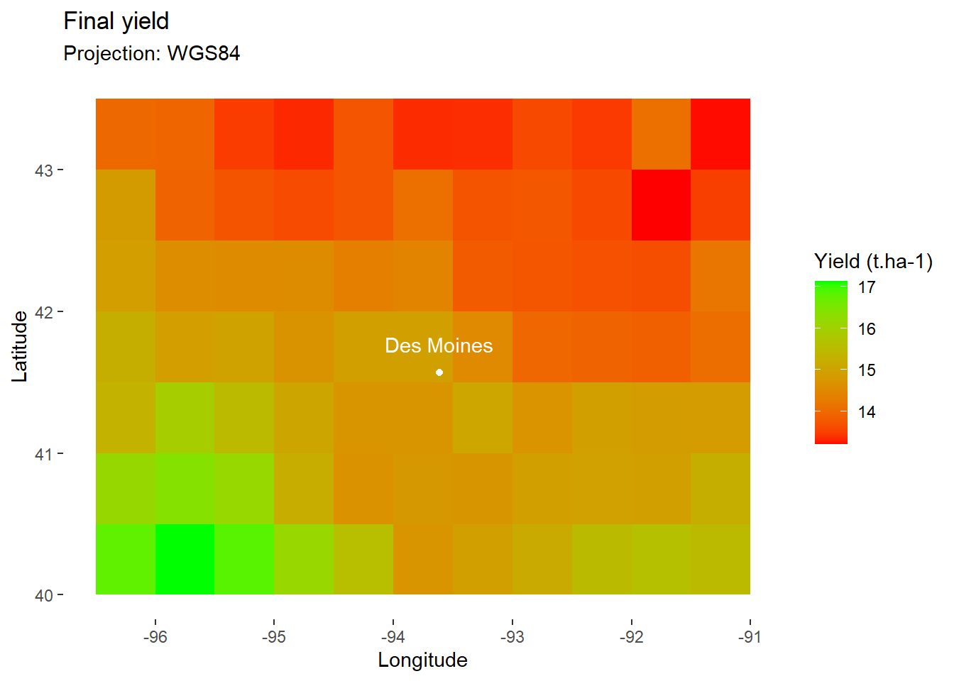
2. Evaluate the validity of the model
One common measure of the differences between values predicted by a model and the values observed is the Root Mean Square Error (RMSE). The calculation of the RMSE is usually based on field data but, in this case, we will use the results of another crop model as reference.
In our case, it is calculated as follows:
\[ \quad\text{(Eq. 1)}\quad RMSE = \sqrt\frac{\sum_{i=1}^N(Y_{i}^{Our Model}-Y_{i}^{Ref Model})^{2}}{N}\]
With:
\(Y_{i}^{OurModel}\): final yield estimated by our model (\(t.ha^{-1}\))
\(Y_{i}^{RefModel}\): final yield estimated by reference model (\(t.ha^{-1}\))
\(N\): total number of simulations
2.1. Load reference data
We will compare the results of our model with results from the Lund-Potsdam-Jena managed land model. Outputs of this reference model for our study area are available here.
# Load data
reference <- read.table(file="Yields_Iowa_lpjml.csv", header=TRUE, sep=",",dec=".")
head(reference)
## X lon lat yield_t
## 1 1 -96.25 40.25 10.154525
## 2 2 -95.75 40.25 10.012679
## 3 3 -95.25 40.25 10.053258
## 4 4 -94.75 40.25 9.989664
## 5 5 -94.25 40.25 10.041997
## 6 6 -93.75 40.25 10.114156As you can see, there is no “day_number” variable in this table, which only gives the final yield values. Before comparing these yields with the outputs of our model, we will slightly modify this table, by keeping only the necessary columns and changing the name of the variable where yields are stored.
# Prepare data: select required columns and rename yield
reference<-reference%>%
  select(
    lon=lon,
    lat=lat,
    grain_reference=yield_t
  )

head(reference)
## lon lat grain_reference
## 1 -96.25 40.25 10.154525
## 2 -95.75 40.25 10.012679
## 3 -95.25 40.25 10.053258
## 4 -94.75 40.25 9.989664
## 5 -94.25 40.25 10.041997
## 6 -93.75 40.25 10.1141562.2. Compare model to reference
Now we are ready to compare the results of our model to the reference. In the ‘pipes’ below, we will start by applying our model with median values for both \(C\) and \(RUE\) parameters and only keep the results for the harvest day. Then, we will merge this table with those of the reference model (based on latitude and longitude coordinates). Finally, for each cell, we will calculate the gap between the results of our model and the reference.
comp <- model_whole_fun(          # Apply model with median values for C and RUE
  data=data, C=0.2, RUE=2
  )%>%
  filter(
    day_number==day_harvest       # Keep only final results
  )%>%
  merge(
    reference,by=c('lon','lat')   # Add results of the reference model
  )%>%
  mutate(
    gap=grain_t-grain_reference   # Compute gap between model and ref
  )%>%
  mutate(
    gap_square=gap*gap            # Compute square gap
  )%>%                            # (will be useful for RMSE computation)
  select(
    lon,lat,gap,gap_square
  )

head(comp)
## lon lat gap gap_square
## 1 -91.25 40.25 5.938888 35.27039
## 2 -91.25 40.75 6.052363 36.63110
## 3 -91.25 41.25 5.643455 31.84859
## 4 -91.25 41.75 4.750789 22.56999
## 5 -91.25 42.25 4.845909 23.48284
## 6 -91.25 42.75 4.289735 18.40182We may now map the gap between our model and the reference.
map_gap<-ggplot(
  data=comp,       # Keep only final values
  aes(x=lon,y=lat,fill=gap))+                   # Fill according to final yield
  geom_tile()+                                      # Add tiles
  labs(
    title="Gap between model and reference",
    subtitle="Projection: WGS84",
    x="Longitude",
    y="Latitude",
    fill="Gap (t.ha-1)"                           # Specify fill legend
  )+
  theme_custom

map_gap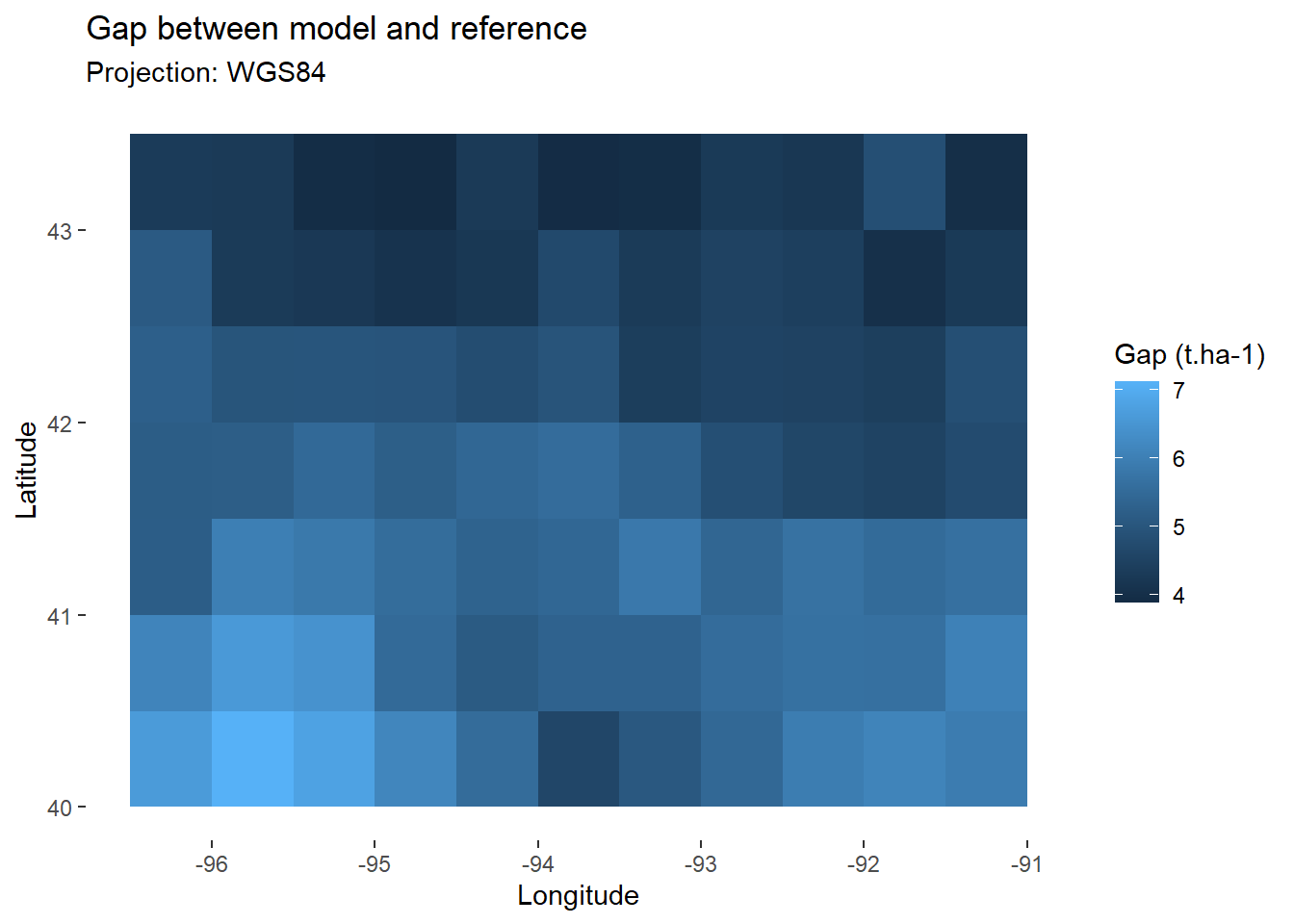
Overall, we see that our model tends to overestimate yields. To know the average error for the whole area, we can calculate the RMSE, as specified in (Eq. 1).
rmse <- comp%>%
  mutate(
    cum_gap=cumsum(gap_square)      # Cumulative sum of square error
  )%>%
  tail(1)%>%                        # Keep only the last line
  mutate(
    RMSE=sqrt(cum_gap/nrow(comp))   # Compute RMSE (see (Eq.1))
  )%>%
  select(RMSE)

head(rmse)
## RMSE
## 77 5.166122So, with this configuration (with median value for \(C\) and \(RUE\)), our model has a mean error of 5t.ha-1 compared to the reference, which is rather substantial. We will try to optimize our model to reduce this error.
3. Model optimization
For the optimization of the model, we will focus on the \(RUE\) parameter, which, as we saw in the second part, was the one that had the most influence on the final result of the model.
3.1. Function creation
In order to facilitate the process, we will create a function that repeats the different steps of the RMSE calculation detailed above. As we want to optimize \(RUE\), we will take this parameter as argument.
optim_fun<-function(RUE_var){

  rmse <- model_whole_fun(          # Apply model with median values for C and RUE
    data=data, C=0.2, RUE=RUE_var
    )%>%
    filter(
      day_number==day_harvest       # Keep only final results
    )%>%
    merge(
      reference,by=c('lon','lat')   # Add results of the reference model
    )%>%
    mutate(
      gap=grain_t-grain_reference   # Compute gap between model and ref
    )%>%
    mutate(
      gap_square=gap*gap            # Compute square gap
    )%>%                            # (will be useful for RMSE computation)
    select(
      lon,lat,gap,gap_square
    )%>%
    mutate(
      cum_gap=cumsum(gap_square)    # Cumulative sum of square error
    )%>%
    tail(1)%>%                      # Keep only the last line
    mutate(
      RMSE=sqrt(cum_gap/nrow(comp)) # Compute RMSE (see (Eq.1))
    )%>%
    select(RMSE)

  return(as.numeric(rmse))

}
This function now allows us to easily calculate the RMSE for different values of \(RUE\).
optim_fun(1)## [1] 2.22229Above, we can see that decreasing the value of RUE from 2 to 1 has halved the error of the model.
3.2. Optimization of RUE
We are now looking for the value of RUE that maximizes the accuracy of the model (that is, the model configuration with the lowest RMSE). To do so, as with the sensitivity analysis (see Part II), we will create an input table with multiple values for RUE.
optim_input<-data.frame(
    RUE_draw=seq(1,3,0.1)       # RUE varies from 1 to 3 with a step of 0.1
  )

head(optim_input)
## RUE_draw
## 1 1.0
## 2 1.1
## 3 1.2
## 4 1.3
## 5 1.4
## 6 1.5Then, we will apply our optimization function to each of these values of \(RUE\). To do so, as for the sentivity analysis, we will use mapply() (note that here we could also use sapply() because our function has only one argument).
optim<-optim_input%>%
  # "Pipe" optimization function to the input data frame:
  mutate(
    rmse=mapply(
      optim_fun,            # Name of the function
      RUE_var=RUE_draw      # Name of the argument
    )
  )

head(optim)
## RUE_draw rmse
## 1 1.0 2.2222895
## 2 1.1 1.5125451
## 3 1.2 0.8422680
## 4 1.3 0.4510416
## 5 1.4 0.8774179
## 6 1.5 1.5519943Looking at the first rows of the table, it would appear that the minimum RMSE is achieved with a \(RUE\) of 1.3. We can now confirm that with a plot.
ggplot(data=optim,aes(x=RUE_draw,y=rmse))+
  geom_point()+
  annotate(
    geom="segment",
    x=1.3,xend=1.3,y=-Inf,yend=Inf,
    color="red")+
  labs(
    title = "Model optimization",
    subtitle = "Choice of RUE minimizing RMSE (RUE=1.3)",
    x="RUE (gDM.MJ-1)",
    y="RMSE (t.ha-1)"
  )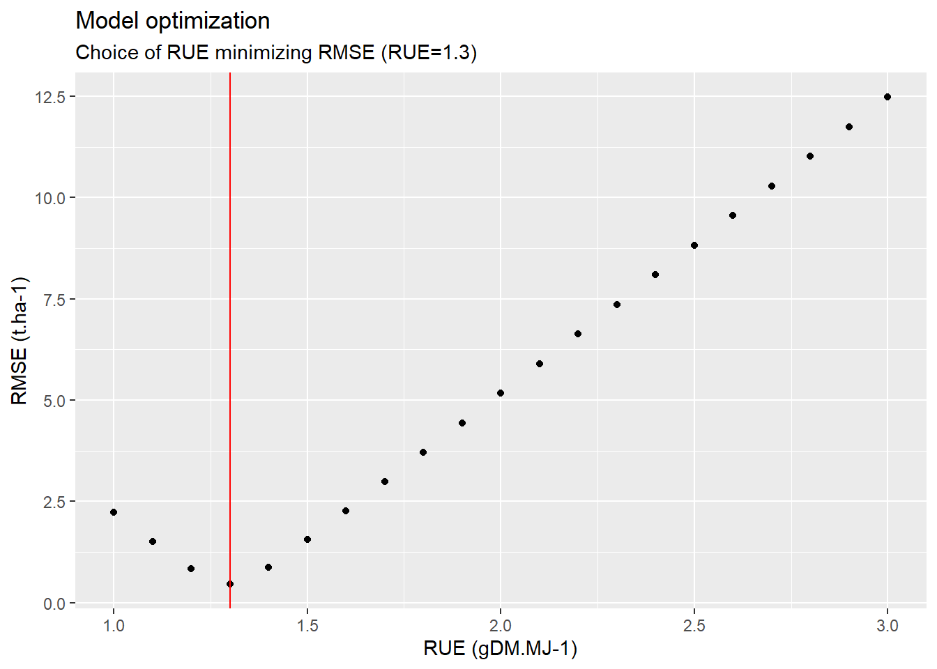
Finally, we can plot the map with the lowest RMSE.
optim_RUE<-1.3
# Apply function with "best" RUE
model_optim <- model_whole_fun(data=data, C=0.2, RUE=optim_RUE)

map_best_yield<-ggplot(
  data=filter(model_optim,day_number==day_harvest),  # Keep only final values
  aes(x=lon,y=lat,fill=grain_t))+                    # Fill according to final yield
  geom_tile()+                                       # Add tiles
  labs(
    title="Best yield estimation",
    subtitle="+/- 0.45 t.ha-1 compared to reference",
    x="Longitude",
    y="Latitude",
    fill="Yield (t.ha-1)"                            # Specify fill legend
  )+
  scale_fill_gradient(
    low="red",
    high="green"
  )+
  DM_loc+
  DM_name+
  theme_custom


map_best_yield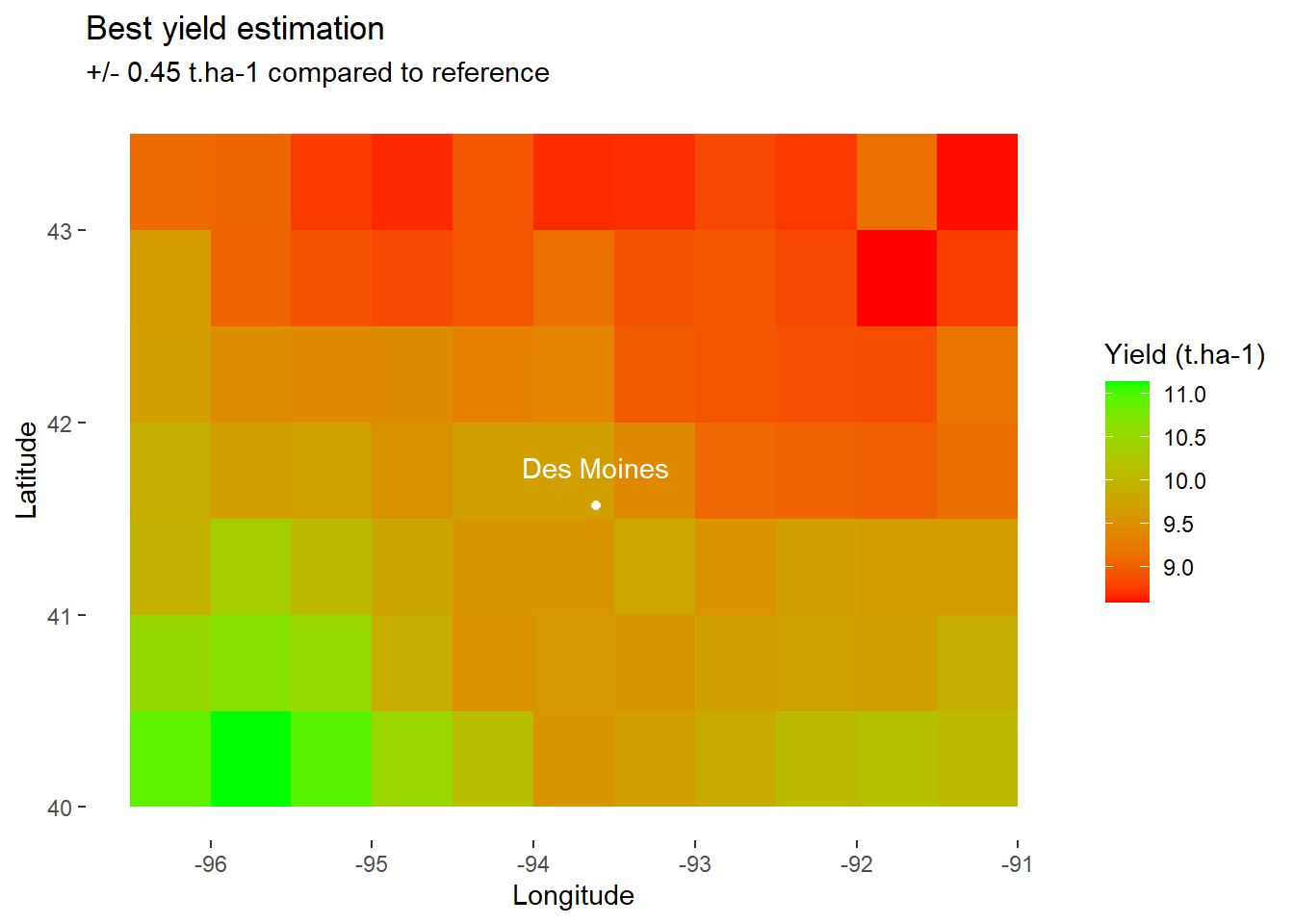
Acknowledgement
My deepest thanks to Bruno Ringeval who provided the data for this tutorial.
Reference
- Ringeval, B. et al. (2021). Potential yield simulated by global gridded crop models: using a process-based emulator to explain their differences. Geosci. Model Dev., 14, 1639–1656. https://doi.org/10.5194/gmd-14-1639-2021