In this post, we will perform a Principal Component Analysis (PCA) to explore the evolution of songs’ features over the years. We will see how we can use the {tidyverse} tools and syntax to perform this PCA.
For this, we will use the TidyTuesday dataset of Top 100 Billboard. To this data set is associated a characterization of the songs according to several features (danceability, mode, tempo…), provided by the Spotify API.
1. Data preparation
# Load data
# Billbord ranking
billboard <- readr::read_csv('https://raw.githubusercontent.com/rfordatascience/tidytuesday/master/data/2021/2021-09-14/billboard.csv')
# Songs features based on Spotify API
features <- readr::read_csv('https://raw.githubusercontent.com/rfordatascience/tidytuesday/master/data/2021/2021-09-14/audio_features.csv')

head(features)
## # A tibble: 6 x 22
## song_id performer song spotify_genre spotify_track_id spotify_track_pr~
## <chr> <chr> <chr> <chr> <chr> <chr>
## 1 -twistin~ Bill Blac~ -twist~ [] <NA> <NA>
## 2 ¿Dònde E~ Augie Rios ¿Dònde~ ['novelty'] <NA> <NA>
## 3 ......An~ Andy Will~ ......~ ['adult stand~ 3tvqPPpXyIgKrm4~ https://p.scdn.c~
## 4 ...And T~ Sandy Nel~ ...And~ ['rock-and-ro~ 1fHHq3qHU8wpRKH~ <NA>
## 5 ...Baby ~ Britney S~ ...Bab~ ['dance pop',~ 3MjUtNVVq3C8Fn0~ https://p.scdn.c~
## 6 ...Ready~ Taylor Sw~ ...Rea~ ['pop', 'post~ 2yLa0QULdQr0qAI~ <NA>
## # ... with 16 more variables: spotify_track_duration_ms <dbl>,
## # spotify_track_explicit <lgl>, spotify_track_album <chr>,
## # danceability <dbl>, energy <dbl>, key <dbl>, loudness <dbl>, mode <dbl>,
## # speechiness <dbl>, acousticness <dbl>, instrumentalness <dbl>,
## # liveness <dbl>, valence <dbl>, tempo <dbl>, time_signature <dbl>,
## # spotify_track_popularity <dbl>For the next part of our analysis we will look at the evolution of songs’ features over the years. To do this, we need to create a column with the year of songs’ creation, using {tidyverse} tools. Then, we will add this new column to songs’ features data.
library(tidyverse)

bill_prep<-billboard%>%
  # Keep only 1st appearance on Billboard
  filter(
    (weeks_on_chart==1)&(instance==1)
  )%>%
  # Add Year column
  mutate(year=format(
    as.Date(week_id,"%m/%d/%Y"),format="%Y")
  )%>%
  # Set year as numeric
  mutate(year=as.numeric(year))

# Add year to songs' features data
features_prep<-features%>%
  left_join(bill_prep,by="song_id")
2. Data cleaning and PCA
First, we will select the variables on interest for the PCA, plus one additional variable (year of creation of the song).
PCA_data<-features_prep%>%
  select(
    # Variables of interest for PCA
    c(danceability,energy,instrumentalness,
      key,acousticness,mode,valence,tempo,
      time_signature,speechiness,loudness,liveness,
    # Add year as supplementary variable
      year
    )
  )%>%
  # Remove rows with NA
  drop_na()
We are now ready to perform the PCA.
PCA <-PCA_data%>%
  select(-year)%>%
  # Perform PCA with scaled variables
  prcomp(scale = TRUE)
Now, we need the {broom} extension to access the results of prcomp() with the {tidyverse} syntax. After loading {broom}, you can use the tidy() function to access the results of the PCA such as eigenvalues.
library(broom)

PCA%>%
  tidy(matrix = "eigenvalues")
## # A tibble: 12 x 4
## PC std.dev percent cumulative
## <dbl> <dbl> <dbl> <dbl>
## 1 1 1.61 0.217 0.217
## 2 2 1.17 0.114 0.331
## 3 3 1.09 0.0993 0.431
## 4 4 1.04 0.0893 0.520
## 5 5 1.01 0.0850 0.605
## 6 6 0.980 0.0801 0.685
## 7 7 0.965 0.0776 0.762
## 8 8 0.928 0.0717 0.834
## 9 9 0.894 0.0666 0.901
## 10 10 0.760 0.0482 0.949
## 11 11 0.660 0.0363 0.985
## 12 12 0.420 0.0147 1Here we can see that the first Principal Component (PC) accounts for 22% of the overall variability (11% for PC2).
3. Plot of individuals
# Add 'year' variable to plot results
PCA_indiv<-PCA%>%
  broom::augment(PCA_data)

# Plot of individuals
ggplot(
  data=PCA_indiv,
  aes(.fittedPC1, .fittedPC2,color=year))+
  geom_point()+
  labs(
    title = 'Plot of individuals',
    subtitle = 'Color shows year of song creation',
    x='PC1 (22%)',
    y='PC2 (11%)',
    color='Year'
  )+
  theme_minimal()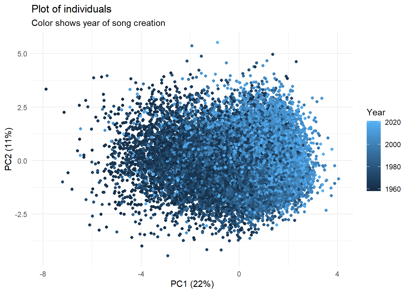
It seems that PC1 distinguishes well the songs according to their years of creation. We will now see which variables contribute the most to this axis.
4. Plot of variables
Variable coordinates are stored in the “rotation” matrix. We can extract these coordinates as follows:
PCA_var<-PCA %>%
  # Extract variable coordinates
  tidy(matrix = "rotation") %>%
  # Format table form long to wide
  pivot_wider(names_from = "PC", names_prefix = "PC", values_from = "value")%>%
  # Rename column with variable names
  rename(Variable=column)%>%
  # 'Clean' variable names
  # Upper case on first letter
  mutate(Variable=stringr::str_to_title(Variable))%>%
  # Change '_' for space
  mutate(Variable=stringr::str_replace_all(Variable,"_"," "))

head(PCA_var)
## # A tibble: 6 x 13
## Variable PC1 PC2 PC3 PC4 PC5 PC6 PC7 PC8
## <chr> <dbl> <dbl> <dbl> <dbl> <dbl> <dbl> <dbl> <dbl>
## 1 Danceability 0.331 -0.542 0.00516 0.164 -0.133 -0.0879 0.140 0.155
## 2 Energy 0.525 0.234 -0.161 -0.0851 0.0569 0.145 -0.0808 0.114
## 3 Instrumental~ -0.0422 -0.195 -0.304 -0.521 0.0581 -0.327 -0.635 0.106
## 4 Key 0.0382 -0.114 0.382 -0.559 0.233 0.395 0.248 -0.245
## 5 Acousticness -0.461 -0.0693 -0.0153 -0.0601 -0.212 0.0326 0.149 -0.0402
## 6 Mode -0.160 0.207 -0.497 0.329 -0.0900 0.107 0.0612 -0.220
## # ... with 4 more variables: PC9 <dbl>, PC10 <dbl>, PC11 <dbl>, PC12 <dbl>We may now plot the variables.
# Load ggrepel to avoid variable names to overlap
library(ggrepel)

var<-ggplot(data=PCA_var,aes(PC1, PC2)) +
  # Add variables arrows
  geom_segment(
    xend = 0, yend = 0,
    arrow = arrow(
      length = unit(0.03, "npc"),
      ends = "first"
    )
  )+
  # Add variables names
  geom_text_repel(
    aes(label = Variable),
    hjust = 1,size=3,
    min.segment.length = Inf,
    nudge_x=0.01,nudge_y=0.01
  ) +
  coord_fixed()+
  labs(
    title = 'Plot of variables',
    x='PC1 (22%)',
    y='PC2 (11%)',
    color='Year'
  )+
  theme_minimal()

var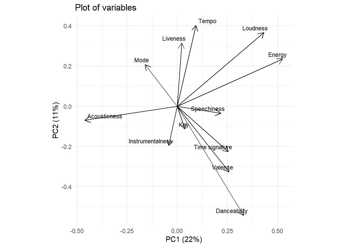
Now we will add year (which was not used for the PCA) as an additional variable on the graph of variables. To do so we will calculate the coordinates of year on the different axes of the PCA.
year_coord<-as.data.frame(
  # Calculate correlation of year with PCA axis
  cor(PCA_data$year,PCA$x)
  )%>%
  # Add name of the variable
  mutate(Variable="Year")

year_coord
## PC1 PC2 PC3 PC4 PC5 PC6 PC7
## 1 0.4652744 0.1592881 0.3657629 0.2336913 0.1282045 -0.1212724 -0.1761371
## PC8 PC9 PC10 PC11 PC12 Variable
## 1 -0.02687627 -0.09279391 0.1115629 0.221641 0.04197899 YearWe may now add this additional variable to the plot of variables.
var+
  geom_segment(
    data=year_coord,
    color="red",
    xend = 0, yend = 0,
    arrow = arrow(
      length = unit(0.03, "npc"),
      ends = "first"
    )
  )+
  geom_text_repel(
    data=as.data.frame(year_coord),
    aes(label = Variable),
    color="red",hjust = 1,size=3,
    min.segment.length = Inf,
    nudge_x=0.02,nudge_y=-0.02
  )+
  labs(
    subtitle="Year as additional variable"
  )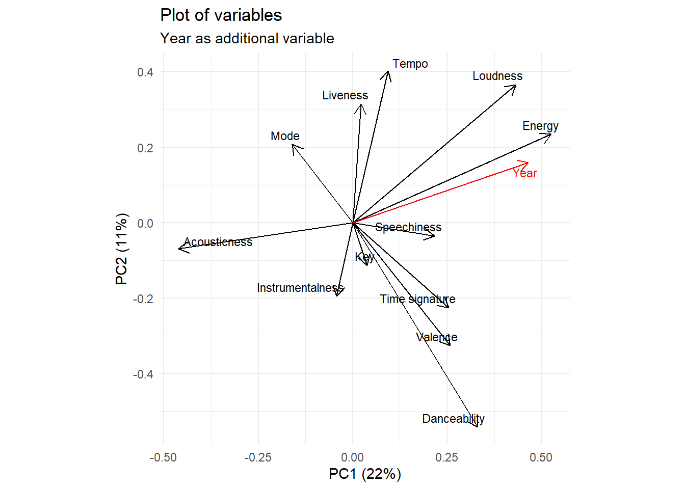
We can see that the “Energy” variable is the most strongly correlated with the “Year” variable: Billboard hits tend to become more and more energetic over the years.
5. Add name of individuals
Finally, you may also add labels to the plot of individuals, to identify some specific points. This is what has been done below to identify the most popular songs in the same dataset.
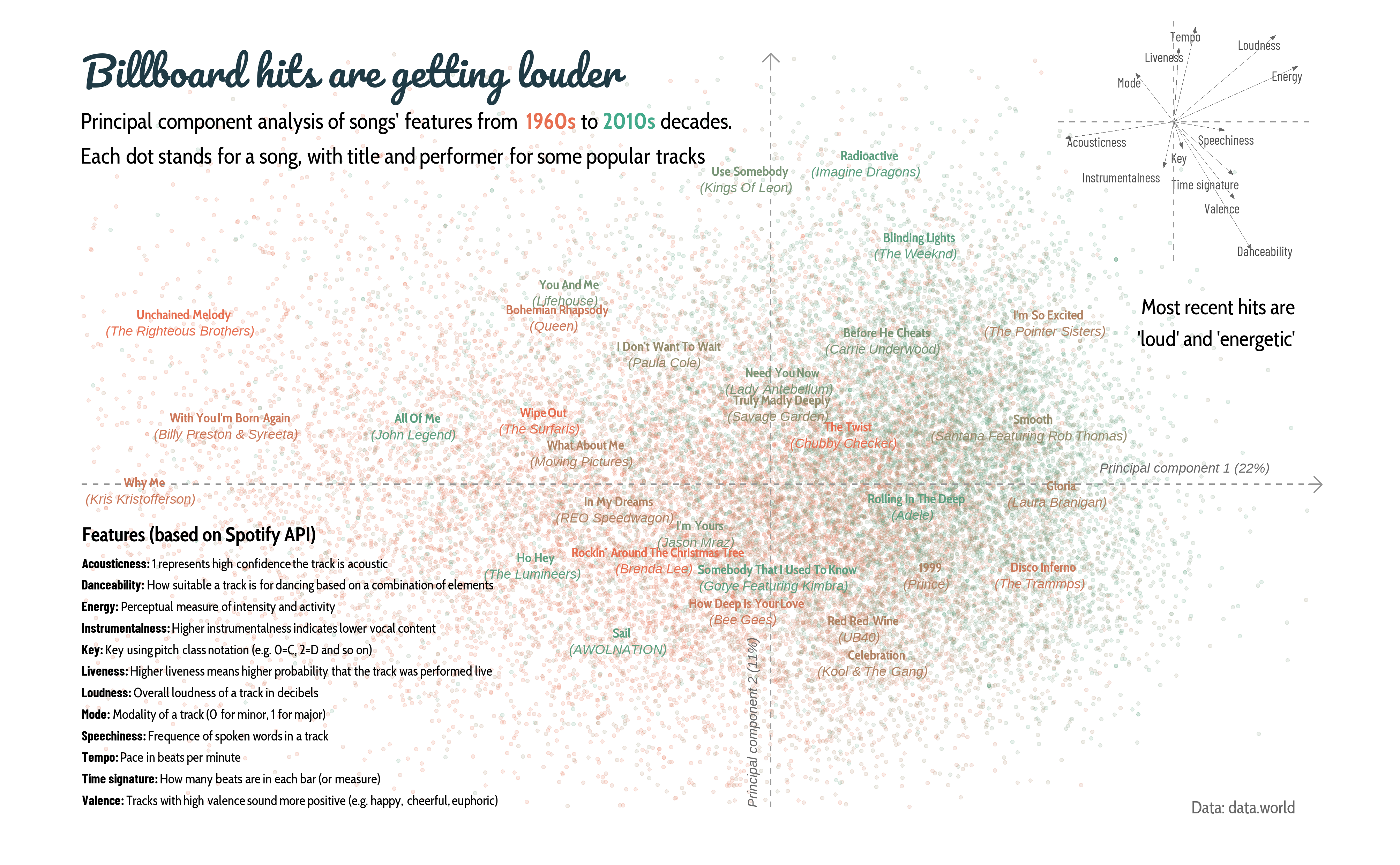
You may find the full code for this example here.
References
Data set: Mock T., Tidy Tuesday
Useful reference for PCA with {tidyverse}: Wilke C.O., PCA tidyverse style