The {gt} extension already allowed to easily create tables from raw dataset, but now the {gtExtras} extension adds many customization options. Here we will illustrate the possibilities of these packages with TidyTuesday dataset on Tour de France riders, extracted from Alastair Rushworth’s {tdf} extension.
1. Tables with text
We will start by loading the data.
library(tidyverse)
# Load data:
# Whole race winners
tdf_winners <- readr::read_csv('https://raw.githubusercontent.com/rfordatascience/tidytuesday/master/data/2020/2020-04-07/tdf_winners.csv')
# Stages winners
tdf_stages <- readr::read_csv('https://raw.githubusercontent.com/rfordatascience/tidytuesday/master/data/2020/2020-04-07/tdf_stages.csv')

head(tdf_stages)
## # A tibble: 6 x 8
## Stage Date Distance Origin Destination Type Winner Winner_Country
## <chr> <date> <dbl> <chr> <chr> <chr> <chr> <chr>
## 1 1 2017-07-01 14 Düsseldorf Düsseldorf Indi~ Gerai~ GBR
## 2 2 2017-07-02 204. Düsseldorf Liège Flat~ Marce~ GER
## 3 3 2017-07-03 212. Verviers Longwy Medi~ Peter~ SVK
## 4 4 2017-07-04 208. Mondorf-les-Bains Vittel Flat~ Arnau~ FRA
## 5 5 2017-07-05 160. Vittel La Planche~ Medi~ Fabio~ ITA
## 6 6 2017-07-06 216 Vesoul Troyes Flat~ Marce~ GERAs a first example, we will make a table with the stage winners of a given year: 1961. We will see later why I chose this year…
tdf_61 <- tdf_stages%>%
  # Create year column from Date
  mutate(year = lubridate::year(Date))%>%
  # Keep only 1961 data
  filter(year==1961)%>%
  # Remove year column
  select(-year)
We will now load the {gt} package to format our first table. One of the main advantages of {gt} is that it fits perfectly into tidyverse pipes: with just have to add the gt() function to create a table.
# Load {gt}
library(gt)

# Make table with gt()
tab<-tdf_61 %>%
  # Keep only first 6 rows as example
  head(6)%>%
  # Make table
  gt()

tab| Stage | Date | Distance | Origin | Destination | Type | Winner | Winner_Country |
|---|---|---|---|---|---|---|---|
| 1a | 1961-06-25 | 136.5 | Rouen | Versailles | Plain stage | André Darrigade | FRA |
| 1b | 1961-06-25 | 28.5 | Versailles | Versailles | Individual time trial | Jacques Anquetil | FRA |
| 2 | 1961-06-26 | 230.5 | Pontoise | Roubaix | Plain stage | André Darrigade | FRA |
| 3 | 1961-06-27 | 197.5 | Roubaix | Charleroi | Plain stage | Emile Daems | BEL |
| 4 | 1961-06-28 | 237.5 | Charleroi | Metz | Plain stage | Anatole Novak | FRA |
| 5 | 1961-06-29 | 221.0 | Metz | Strasbourg | Stage with mountain(s) | Louis Bergaud | FRA |
Once the table is created, we can use the pipe operator %>% to add few functions to customize the table. Here are some examples of how to add a title or format the columns:
tab<-tab %>%
  # Add title and subtitle
  tab_header(
    title = "Stage winners",
    # Use markdown syntax with md()
    subtitle = md("Tour de France **1961**")
  )%>%
  # Fomat date without year information
  fmt_date(
    columns = Date,
    date_style = 9
  )%>%
  # Format distance without decimal
  fmt_number(
    columns = Distance,
    decimals = 0,
    # Add 'km' as suffix
    pattern = "{x} km"
  )%>%
  # Rename column
  cols_label(
    Winner_Country = "Nationality"
  )

tab| Stage winners | |||||||
|---|---|---|---|---|---|---|---|
| Tour de France 1961 | |||||||
| Stage | Date | Distance | Origin | Destination | Type | Winner | Nationality |
| 1a | 25 juin | 136 km | Rouen | Versailles | Plain stage | André Darrigade | FRA |
| 1b | 25 juin | 28 km | Versailles | Versailles | Individual time trial | Jacques Anquetil | FRA |
| 2 | 26 juin | 230 km | Pontoise | Roubaix | Plain stage | André Darrigade | FRA |
| 3 | 27 juin | 198 km | Roubaix | Charleroi | Plain stage | Emile Daems | BEL |
| 4 | 28 juin | 238 km | Charleroi | Metz | Plain stage | Anatole Novak | FRA |
| 5 | 29 juin | 221 km | Metz | Strasbourg | Stage with mountain(s) | Louis Bergaud | FRA |
If you like customization, the {gt} extension allows to change the appearance of each cell (color, background, font, border…). Using the tab_style() function, you may customize the title as follows:
tab %>%
  tab_style(
    # Select object to modify
    locations = cells_title(groups = 'title'),
    # Specify text style
    style = list(
      cell_text(
        font=google_font(name = 'Bebas Neue'),
        size='xx-large',
        color='indianred'
)))| Stage winners | |||||||
|---|---|---|---|---|---|---|---|
| Tour de France 1961 | |||||||
| Stage | Date | Distance | Origin | Destination | Type | Winner | Nationality |
| 1a | 25 juin | 136 km | Rouen | Versailles | Plain stage | André Darrigade | FRA |
| 1b | 25 juin | 28 km | Versailles | Versailles | Individual time trial | Jacques Anquetil | FRA |
| 2 | 26 juin | 230 km | Pontoise | Roubaix | Plain stage | André Darrigade | FRA |
| 3 | 27 juin | 198 km | Roubaix | Charleroi | Plain stage | Emile Daems | BEL |
| 4 | 28 juin | 238 km | Charleroi | Metz | Plain stage | Anatole Novak | FRA |
| 5 | 29 juin | 221 km | Metz | Strasbourg | Stage with mountain(s) | Louis Bergaud | FRA |
You may now try to customize a few parts of the table according to your taste! To help you select the elements you want to modify, here is a table summarizing the different parts of the table:
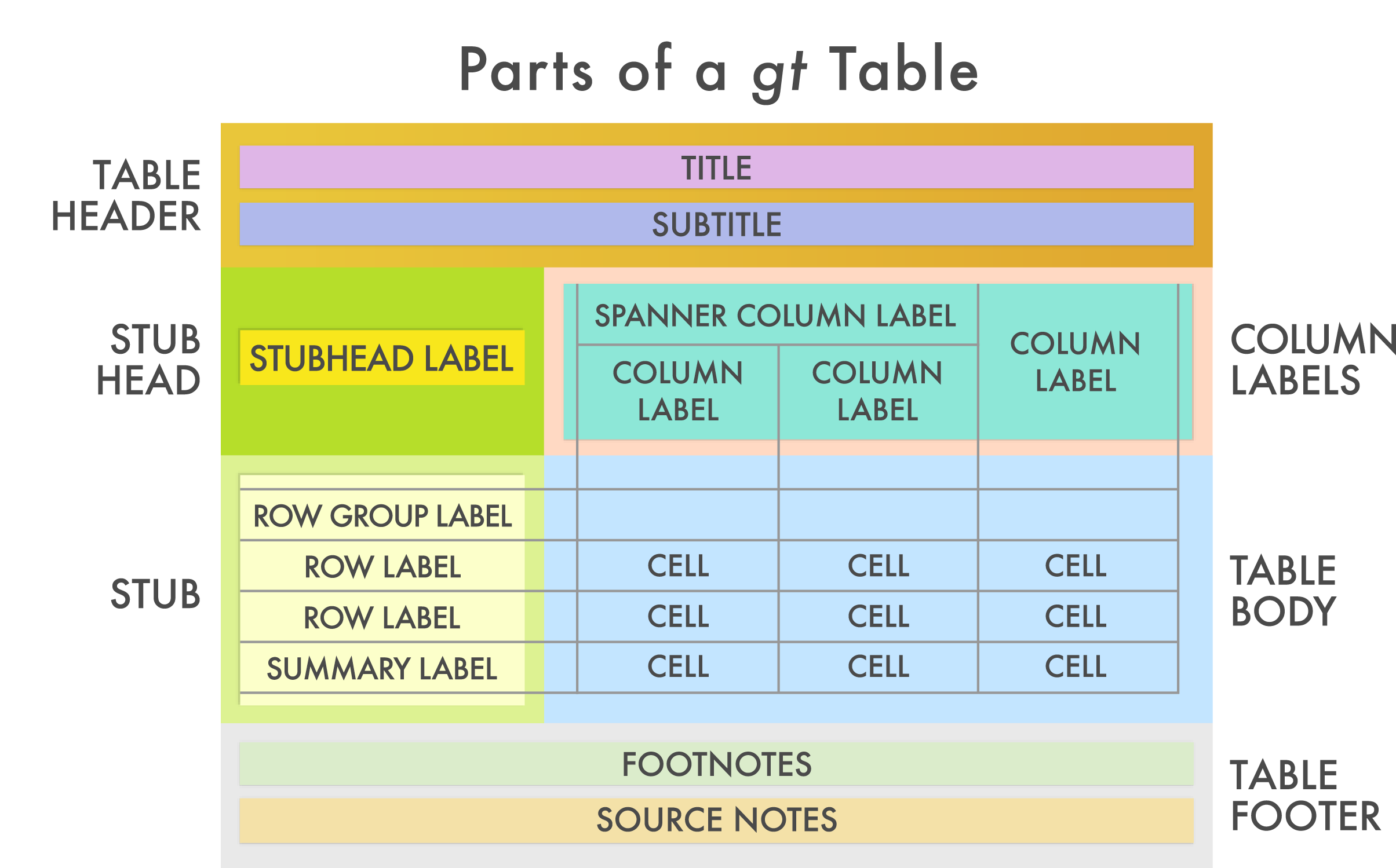
{gt} tables structure (Image credit: Introduction to creating {gt} tables)
You need to specify the name of the element of the table that you want to modifiy, after “cells_”, in the locations argument. These helper functions to target the location cells associated with the styling are summarized here.
But, as you can see, it can be tedious to modify each part of the table in this way. Fortunately, the new {gtExtras} extension allows to use predefined themes.
# Install gtExtras
# remotes::install_github("jthomasmock/gtExtras")

# Load extension
library(gtExtras)
# Apply 'New York Times' theme
tab<-tab%>%
  gtExtras::gt_theme_nytimes()

tab| Stage winners | |||||||
|---|---|---|---|---|---|---|---|
| Tour de France 1961 | |||||||
| Stage | Date | Distance | Origin | Destination | Type | Winner | Nationality |
| 1a | 25 juin | 136 km | Rouen | Versailles | Plain stage | André Darrigade | FRA |
| 1b | 25 juin | 28 km | Versailles | Versailles | Individual time trial | Jacques Anquetil | FRA |
| 2 | 26 juin | 230 km | Pontoise | Roubaix | Plain stage | André Darrigade | FRA |
| 3 | 27 juin | 198 km | Roubaix | Charleroi | Plain stage | Emile Daems | BEL |
| 4 | 28 juin | 238 km | Charleroi | Metz | Plain stage | Anatole Novak | FRA |
| 5 | 29 juin | 221 km | Metz | Strasbourg | Stage with mountain(s) | Louis Bergaud | FRA |
Seven themes are available with {gtExtras}.
We are almost done with this first table. Now it is time to see why I select the stage winnrs of year 1961 as an example. With gt_highlight_rows(), we may highlight the name of one rider.
tab%>%
  gtExtras::gt_highlight_rows(
    # Row to highlight
    rows = 5,
    # Background color
    fill = "lightgrey",
    # Bold for target column only
    bold_target_only = TRUE,
    # Select target column
    target_col = Winner
)| Stage winners | |||||||
|---|---|---|---|---|---|---|---|
| Tour de France 1961 | |||||||
| Stage | Date | Distance | Origin | Destination | Type | Winner | Nationality |
| 1a | 25 juin | 136 km | Rouen | Versailles | Plain stage | André Darrigade | FRA |
| 1b | 25 juin | 28 km | Versailles | Versailles | Individual time trial | Jacques Anquetil | FRA |
| 2 | 26 juin | 230 km | Pontoise | Roubaix | Plain stage | André Darrigade | FRA |
| 3 | 27 juin | 198 km | Roubaix | Charleroi | Plain stage | Emile Daems | BEL |
| 4 | 28 juin | 238 km | Charleroi | Metz | Plain stage | Anatole Novak | FRA |
| 5 | 29 juin | 221 km | Metz | Strasbourg | Stage with mountain(s) | Louis Bergaud | FRA |
Anatole Novak is my grand father. He won one Tour de France stage in 1961, so this is the reason I chose this year as an example. In his career, he also helped Anquetil win several Tour de France. We will see how many in the next table!
2. Add images to table
In this second part, we will see more formatting options, in particular how we can add images to a table.
We will now look at the riders who have won the most Tour de France. This information may be extracted from the tdf_winners dataset:
# Data preparation:
most_wins<-tdf_winners%>%
  # Remove Armstrong (convicted for drug use)
  filter(winner_name!="Lance Armstrong")%>%
  # Keep only one spelling for Indurain
  mutate(winner_name=case_when(
    winner_name=='Miguel Induráin'~'Miguel Indurain',
    TRUE~winner_name
  ))%>%
  # Add variable to count titles
  mutate(ct=1)%>%
  # Group by winner name
  group_by(winner_name)%>%
  summarize(
    # Count titles
    Titles=sum(ct),
    # Add nationality
    Country=nationality[1],
    # Add nickname
    Nickname=nickname[1])%>%
  # Keep only winners with 3 titles or more
  filter(Titles>2)%>%
  # Sort by descending order
  arrange(-Titles)

most_wins
## # A tibble: 8 x 4
## winner_name Titles Country Nickname
## <chr> <dbl> <chr> <chr>
## 1 Bernard Hinault 5 France Le Blaireau (The Badger), Le Patron (T~
## 2 Eddy Merckx 5 Belgium The Cannibal
## 3 Jacques Anquetil 5 France Monsieur Chrono, Maître Jacques
## 4 Miguel Indurain 5 Spain Miguelón, Big Mig (English)
## 5 Chris Froome 4 Great Britain Froomey
## 6 Greg LeMond 3 United States L’Americain, LeMonster
## 7 Louison Bobet 3 France Louison, Zonzon
## 8 Philippe Thys 3 Belgium Le basset (The Basset Hound)We are almost ready to convert this dataset into a {gt} table. Before that, we will rename the first column and reorder the others. Thus, the operations carried out on the data tibble will be reproduced on the {gt} table, which will keep the same column order. We will also clean up the list of nicknames.
# Data preparation:
most_wins<-most_wins%>%
  # Ordering columns
  select(
    Rider=winner_name,
    Nickname,Country,Titles)%>%
  # Cleaning nicknames
  mutate(Nickname=case_when(
    str_detect(Rider,'Hinault')~'The Badger',
    str_detect(Rider,'Anquetil')~'Maître Jacques',
    str_detect(Rider,'Indurain')~'Miguelón',
    str_detect(Rider,'LeMond')~"The American",
    str_detect(Rider,'Bobet')~'Zonzon',
    str_detect(Rider,'Thys')~'The Basset Hound',
    TRUE~Nickname
  ))
Preparation of the dataset is now complete, we may create the table. At the same time, we will discover a new function, gt_merge_stacks(), which allows to merge two columns (here riders name and nickname).
most_wins%>%
  gt()%>%
  tab_header(
    title = "Most sucessful riders in the Tour de France"
  )%>%
  gtExtras::gt_theme_nytimes()%>%
  # Merge riders' name and nickname on same column
gtExtras::gt_merge_stack(col1 = Rider, col2 = Nickname)| Most sucessful riders in the Tour de France | ||
|---|---|---|
| Rider | Country | Titles |
Bernard Hinault
The Badger |
France | 5 |
Eddy Merckx
The Cannibal |
Belgium | 5 |
Jacques Anquetil
Maître Jacques |
France | 5 |
Miguel Indurain
Miguelón |
Spain | 5 |
Chris Froome
Froomey |
Great Britain | 4 |
Greg LeMond
The American |
United States | 3 |
Louison Bobet
Zonzon |
France | 3 |
Philippe Thys
The Basset Hound |
Belgium | 3 |
The next column to customize is now the riders nationality: we will replace the name of the countries by an image of their respective flags. We can not do this directly from the table, we have to go back to the dataset to replace the name of the countries by the link to the flag image.
most_wins <- most_wins%>%
  mutate(Country = case_when(
    str_detect(Country,'France') ~ 'https://raw.githubusercontent.com/BjnNowak/TdF/main/fr.png',
    str_detect(Country,'Belgium') ~ 'https://raw.githubusercontent.com/BjnNowak/TdF/main/be.png',
    str_detect(Country,'Great Britain') ~ 'https://raw.githubusercontent.com/BjnNowak/TdF/main/uk.png',
    str_detect(Country,'Spain') ~ 'https://raw.githubusercontent.com/BjnNowak/TdF/main/sp.png',
    str_detect(Country,'United States') ~ 'https://raw.githubusercontent.com/BjnNowak/TdF/main/us.png'
  ))
Flag images can then be displayed in the table with the gt_img_rows() function.
tab2 <- most_wins%>%
  gt()%>%
  tab_header(
    title = "Most sucessful riders in the Tour de France"
  )%>%
  gtExtras::gt_theme_nytimes()%>%
  gtExtras::gt_merge_stack(col1 = Rider, col2 = Nickname)%>%
  # Add flag images
  gtExtras::gt_img_rows(columns = Country, height = 20)

tab2| Most sucessful riders in the Tour de France | ||
|---|---|---|
| Rider | Country | Titles |
Bernard Hinault
The Badger |
 |
5 |
Eddy Merckx
The Cannibal |
 |
5 |
Jacques Anquetil
Maître Jacques |
|
5 |
Miguel Indurain
Miguelón |
 |
5 |
Chris Froome
Froomey |
 |
4 |
Greg LeMond
The American |
 |
3 |
Louison Bobet
Zonzon |
|
3 |
Philippe Thys
The Basset Hound |
|
3 |
The last column to customize is the one with the number of titles. We could replace it with a barplot with gt_plt_bar(), but we will see the use of graphs in the third and last part. Here, we will replace the number of titles by icons representing a yellow jersey, which designates the leader of the Tour de France. To do so, we will use the gt_fa_repeats() function.
tab2%>%
  gtExtras::gt_fa_repeats(
    column=Titles,
    palette = "orange",
    name = "tshirt",
    align='left'
)| Most sucessful riders in the Tour de France | ||
|---|---|---|
| Rider | Country | Titles |
Bernard Hinault
The Badger |
|
|
Eddy Merckx
The Cannibal |
|
|
Jacques Anquetil
Maître Jacques |
|
|
Miguel Indurain
Miguelón |
|
|
Chris Froome
Froomey |
|
|
Greg LeMond
The American |
|
|
Louison Bobet
Zonzon |
|
|
Philippe Thys
The Basset Hound |
|
|
3. Add plots to table
To start this third part of our tutorial, we will create a new column showing a ‘title timeline’ for each rider. To make a plot from a column, it is generally necessary that this column contains several information. It is therefore necessary to group these data in a list, which will then be called by the function that will create the graph. Moreover, we want these lists to be ‘complete’, so that the data is homogeneous between the different runners. In this case, we will create a variable a variable that takes the value 1 for years with a title, 0 otherwise. To do so, we will use the complete() function. Finally, we will group the data in a list.
# Create a vector with names of riders with most wins
names_most_wins<- most_wins %>%
  pull(Rider)

year_wins<-tdf_winners%>%
  # Rider column with one spelling for Indurain
  mutate(Rider=case_when(
    winner_name=='Miguel Induráin'~'Miguel Indurain',
    TRUE~winner_name
  ))%>%
  # Add ct variable to count years,
  # with 1 for year with a title
  mutate(ct=1)%>%
  # ... and create new rows with ct=0
  # for years with no title
  complete(Rider, edition, fill = list(ct = 0))%>%
  group_by(Rider)%>%
  # Create list for each rider
  summarise(Timeline = list(ct))%>%
  filter(Rider %in% names_most_wins)

year_wins
## # A tibble: 8 x 2
## Rider Timeline
## <chr> <list>
## 1 Bernard Hinault <dbl [106]>
## 2 Chris Froome <dbl [106]>
## 3 Eddy Merckx <dbl [106]>
## 4 Greg LeMond <dbl [106]>
## 5 Jacques Anquetil <dbl [106]>
## 6 Louison Bobet <dbl [106]>
## 7 Miguel Indurain <dbl [106]>
## 8 Philippe Thys <dbl [106]>Once the list is created, we may plot the timeline in a table with gt_sparkline(). With the latest versions of the package, labels may be displayed on the x-axis but they may be turned off with label=FALSE.
year_wins%>%
  gt()%>%
  gtExtras::gt_sparkline(
    # Select column with data
    Timeline,
    # Color for min/max points
    range_colors=c("#ABB4C4","#ef233c"),
    # Line color
    line_color="#DBDFE6",
    # Hide labels
    # (for latest versions of {gtExtras}) only:
    # label=FALSE
    )%>%
  tab_header(title = "Titles timeline")%>%
gtExtras::gt_theme_nytimes()| Titles timeline | |
|---|---|
| Rider | Timeline |
| Bernard Hinault | |
| Chris Froome | |
| Eddy Merckx | |
| Greg LeMond | |
| Jacques Anquetil | |
| Louison Bobet | |
| Miguel Indurain | |
| Philippe Thys | |
As there have been more than 100 editions of the Tour de France, it is difficult to read the timeline precisely, but we can at least compare the periods of activity each rider. For example, Thys was the first to win at least three tours, while Froome is the one who reached this threshold most recently.
As a last example, we will create a barplot with the number of stages won by each rider, as well as the type of stage won (Moutain stage, plain stage or time trial).
most_stages<- tdf_stages %>%
  mutate(Rider=case_when(
    Winner=='Miguel Induráin'~'Miguel Indurain',
    TRUE~Winner
  ))%>%
  filter(Rider %in% names_most_wins)%>%
  # Keep only 3 types of stages:
  # Time trial, mountain or plain
  mutate(TypeClean = case_when(
    str_detect(Type,"trial")~"Time trial",
    str_detect(Type,"mountain")~"Mountain stage",
    str_detect(Type,"Mountain")~"Mountain stage",
    str_detect(Type,"Hilly")~"Mountain stage",
    TRUE~"Plain stage"
  ))%>%
  group_by(Rider,TypeClean) %>%
  mutate(ct=1) %>%
  summarize(
    Wins=sum(ct)
  )%>%
  ungroup()%>%
  # Complete with NA for empty couples {rider*type of stages}
  complete(Rider, TypeClean, fill = list(Wins = NA)) %>%
  group_by(Rider)%>%
  summarise(Stages = list(Wins))
Again, once the list is created, we may plot the number of stages won in a table with gt_plt_bar_stack().
# Set color palette
pal_stages <- c('#264653','#e9c46a','#e76f51')

most_stages %>%
  gt()%>%
  gt_plt_bar_stack(
    # Column with data
    column=Stages,
    # Stacked barplot
    position = 'stack',
    # Set labels and color
    labels = c("Mountain stage", "Plain stage", "Time trial"),
    palette = pal_stages,
    # Barplot width
    width = 60,
    # Same size for all labels
    trim=TRUE
  )%>%
  tab_header(title = "Stages won")%>%
gt_theme_nytimes()| Stages won | |
|---|---|
| Rider | Mountain stage||Plain stage||Time trial |
| Bernard Hinault | |
| Chris Froome | |
| Eddy Merckx | |
| Greg LeMond | |
| Jacques Anquetil | |
| Louison Bobet | |
| Miguel Indurain | |
| Philippe Thys | |
Finally, to group all this information in the same table, we will proceed with joins before creating the table, and then simply use the same functions as previously done to format the columns. It is also a good way to summarize what we have learned.
tab3<-most_wins%>%
  # Join tables
  left_join(year_wins)%>%
  left_join(most_stages)%>%
  # Make table
  gt()%>%
  # Set title
  tab_header(
    title = "Most sucessful riders in the Tour de France"
  )%>%
  # Set theme
  gtExtras::gt_theme_nytimes()%>%
  # Merge riders' name and nickname on same column
  gtExtras::gt_merge_stack(col1 = Rider, col2 = Nickname)%>%
  # Add flag images
  gtExtras::gt_img_rows(columns = Country, height = 20)%>%
  # Add yellow jerseys
  gtExtras::gt_fa_repeats(
    column=Titles,palette = "orange",
    name = "tshirt",align='left'
  )%>%
  # Format timeline
  gtExtras::gt_sparkline(
    Timeline, range_colors=c("#ABB4C4","#ef233c"),
    line_color="#DBDFE6"
  )%>%
  # Format stages won
  gt_plt_bar_stack(
    column=Stages, position = 'stack',
    labels = c("Mountain stage", "Plain stage", "Time trial"),
    palette = pal_stages, width = 60, trim=TRUE
  )

tab3 | Most sucessful riders in the Tour de France | ||||
|---|---|---|---|---|
| Rider | Country | Titles | Timeline | Mountain stage||Plain stage||Time trial |
Bernard Hinault
The Badger |
|
|||
Eddy Merckx
The Cannibal |
|
|||
Jacques Anquetil
Maître Jacques |
|
|||
Miguel Indurain
Miguelón |
|
|||
Chris Froome
Froomey |
|
|||
Greg LeMond
The American |
|
|||
Louison Bobet
Zonzon |
|
|||
Philippe Thys
The Basset Hound |
|
|||
Before you leave, you will find below a slightly more personnal version of this table, with a customized theme. In addition, I added a few words of context in the subtitle, a footnote for additional comments and a source note to details the source of the data. Full code for this version is available here.
| Les forçats de la route | ||||
|---|---|---|---|---|
| Les forçats de la route, translated as Convicts on the road, is a report by Albert Londres about the Tour de France 1924, an annual men's multiple-stage bicycle contest. In this race across France, the leader is designated with the yellow jersey. The first race was organized in 1903 and in 108 editions, only eight riders have won three or more titles.1 | ||||
| Rider | Country | Number of titles |
Titles timeline |
Stages won |
| Mountain stage||Plain stage||Time trial | ||||
Bernard Hinault
The Badger |
|
|||
Eddy Merckx
The Cannibal |
|
|||
Jacques Anquetil
Maître Jacques |
|
|||
Miguel Indurain
Miguelón |
|
|||
Chris Froome
Froomey |
|
|||
Greg LeMond
The American |
|
|||
Louison Bobet
Zonzon |
|
|||
Philippe Thys
The Basset Hound |
|
|||
| Data: Alastair Rushworth & TidyTuesday | Table: @BjnNowak | ||||
|
1
Race not contested from 1915 to 1918 and 1940 to 1946 due to World Wars. |
||||
References
Iannone R. et al. Introduction to creating {gt} Tables
Mock T. {gtExtras}