1. Define plot geometry

After logging into Google Earth Engine, we will start by delimiting the contours of our plot of interest. Create a new Script (left panel) and write the following lines of JavaScript code in the Editor (center panel).

// Create your plot
// (you can also do it manually directly on the map)
var geometry = ee.Geometry.Polygon(
        [[[3.246980338791907, 45.835336025505995],
        [3.247881561020911, 45.83249544350292],
        [3.249383598069251, 45.83285426186172],
        [3.2479673917093876, 45.837279498073954],
        [3.2462507779398564, 45.837458892119855]]]);

As there is an uncertainty on the georeferencing of Sentinel images, I generally use a 20m buffer to make sure to keep only pixels within the plot.

// Apply negative buffer to geometry
var geometryBuff = geometry.buffer(-20)

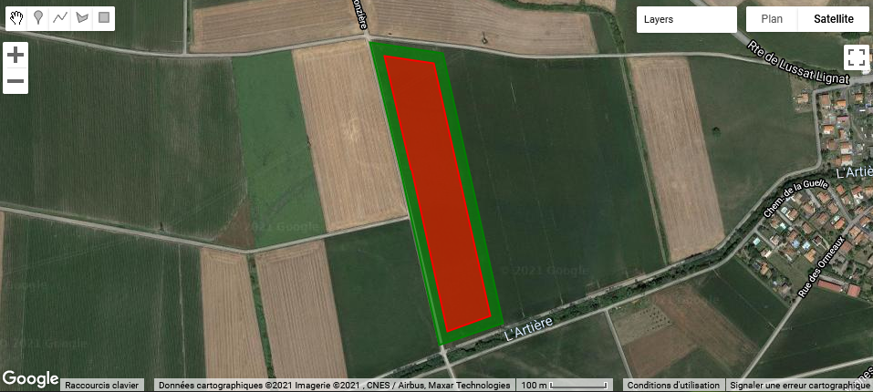
We are now ready to plot these geometries on the map.

// Add plot and buffer to the map
// and specify fill color and layer name
Map.addLayer(geometry,{color:'green'},'Border');
Map.addLayer(geometryBuff,{color:'red'},'Buffer');

// Center map on the plot
Map.centerObject(geometry);

2. Create a collection of clean Sentinel-2 images

When loading Sentinel images, we will remove data biased by shadows or cloud cover. To do this we will use two levels of filtering: first ignore satellite images with cloud cover above a certain threshold and then, for the images that have been retained, keep only the pixels identified as soil or vegetation.

Let’s start by loading a Sentinel image collection that corresponds to our area and period of interest.

// Load image collection of Sentinel-2 imagery
// (choose SR for atmospheric corrections to surface reflectance)
var S2 = ee.ImageCollection('COPERNICUS/S2_SR') 
  // Remove cloudy images from the collection
  .filterMetadata('CLOUDY_PIXEL_PERCENTAGE', 'less_than', 20)
  // Filter to study period
  .filterDate('2019-09-01', '2020-10-01')
  // Filter to plot boundaries
  .filterBounds(geometryBuff);

We will now create a filter to keep only the pixels previously identified as vegetation or bare soil. This information is available in the Scene Classification Layer (SCL) provided with Sentinel-2 data.

// Function to keep only vegetation and soil pixels
function keepFieldPixel(image) {
  // Select SCL layer
  var scl = image.select('SCL'); 
  // Select vegetation and soil pixels
  var veg = scl.eq(4); // 4 = Vegetation
  var soil = scl.eq(5); // 5 = Bare soils
  // Mask if not veg or soil
  var mask = (veg.neq(1)).or(soil.neq(1));
  return image.updateMask(mask);
}

// Apply custom filter to S2 collection
var S2 = S2.map(keepFieldPixel);

In addition, we will also create a filter to mask clouds using the Sentinel-2 QA band, as define in the Earth Engine catalog. We will not apply this filter right away to compare the results later.

// Filter defined here: 
// https://developers.google.com/earth-engine/datasets/catalog/COPERNICUS_S2_SR#description

function maskS2clouds(image) {
  var qa = image.select('QA60');

  // Bits 10 and 11 are clouds and cirrus, respectively.
  var cloudBitMask = 1 << 10;
  var cirrusBitMask = 1 << 11;

  // Both flags should be set to zero, indicating clear conditions.
  var mask = qa.bitwiseAnd(cloudBitMask).eq(0)
      .and(qa.bitwiseAnd(cirrusBitMask).eq(0));

  return image.updateMask(mask);
}

3. Compute NDVI

We will now compute the NDVI based on the red (band 4) and infrared (band 8) reflectance.

// Function to compute NDVI and add result as new band
var addNDVI = function(image) {
return image.addBands(image.normalizedDifference(['B8', 'B4']));
};

// Add NDVI band to image collection
var S2 = S2.map(addNDVI);

One thing to note: GEE will calculate the NDVI for the finest resolution available for bands 4 and 8 (10m in this case).

4. Plot NDVI time series

We can now calculate for each date the average NDVI of the plot with the following function:

var evoNDVI = ui.Chart.image.seriesByRegion(
  S2,                // Image collection
  geometryBuff,      // Region
  ee.Reducer.mean(), // Type of reducer to apply
  'nd',              // Band
  10);               // Scale

We can finally plot the results:

var plotNDVI = evoNDVI                    // Data
    .setChartType('LineChart')            // Type of plot
    .setSeriesNames(['SCL filter only'])
    .setOptions({                         // Plot customization
      interpolateNulls: true,
      lineWidth: 1,
      pointSize: 3,
      title: 'NDVI annual evolution',
      hAxis: {title: 'Date'},
      vAxis: {title: 'NDVI'}
});

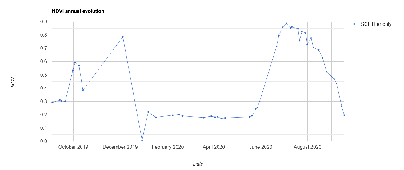
Looking at the plot above, we can see that a late December date seems strange, with a lower NDVI than the usual bare soil NDVI (~0.2). To clean our dataset, we will now apply the second filter defined earlier and specifically designed to remove pixels covered by clouds.

// Apply second filter
var S2 = S2.map(maskS2clouds);

// Plot results
var plotNDVI = ui.Chart.image.seriesByRegion(
  S2, 
  geometryBuff,
  ee.Reducer.mean(),
  'nd',10)
  .setChartType('LineChart')
  .setSeriesNames(['After cloud filter'])
  .setOptions({
    interpolateNulls: true,
    lineWidth: 1,
    pointSize: 3,
    title: 'NDVI annual evolution',
    hAxis: {title: 'Date'},
    vAxis: {title: 'NDVI'},
    series: {0:{color: 'red'}}
  });
  
print(plotNDVI)

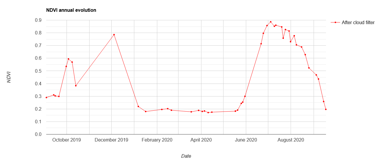
We can see on the plot above that the second filter removed the end of December date. You can consult this post from Philipp Gärtner for more information on the evaluation of cloud cover from the QA60 band.

To come back to our original question, the winter increase in NDVI suggests that a cover crop was sown, then destroyed at the end of December. Next cash crop was sown in following spring.

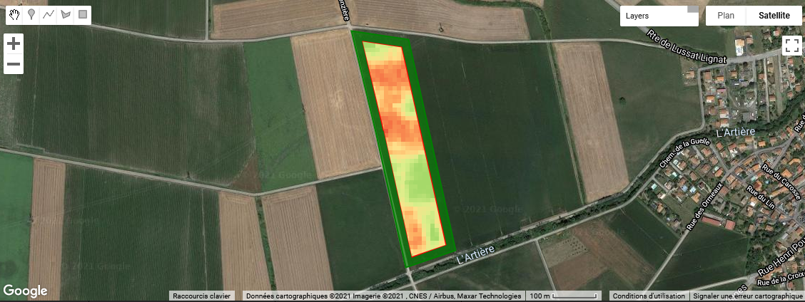
5. Exploring within-field heterogeneities

We can also plot the different NDVI maps obtained. For the sake of simplicity, we will show here only one map: the median NDVI per pixel for the whole study period.

// Extract NDVI band from S2 collection 
var NDVI = S2.select(['nd']);
// Extract median NDVI value for each pixel
var NDVImed = NDVI.median(); 

// Hex values for red to green color palette
var pal = ['#d73027', '#f46d43', '#fdae61', '#fee08b', '#d9ef8b', '#a6d96a'];

// Display NDVI results on map
Map.addLayer(
  NDVImed.clip(geometryBuff),        // Clip map to plot borders
  {min:0.2, max:0.4, palette: pal},  // Specify color palette 
  'NDVI'                             // Layer name
  )

References

• Gärtner P. (2020). How cloudy is my Sentinel-2 image collection? - The ‘QA60’ band gives insights
• Nowak B., Marliac G. and Michaud A. (2021). Estimation of winter soil cover by vegetation before spring-sown crops for mainland France using multispectral satellite imagery