A few months ago we published an article on winter soil cover before spring crops for France. For each plot with spring crops, we used Sentinel-2 multispectral satellite images to estimate winter soil cover through the computation of the Normalized Difference Vegetation Index (NDVI), which is the most commonly used vegetation monitoring index in agriculture.
After some basic elements on the rationale behind NDVI, this tutorial shows:
- (i) how to download the Sentinel-2 images provided free of charge by the European Space Agency (ESA)
- (ii) how to create a NDVI map with the open source software QGIS from these data.
1. Rationale behind NDVI computation
They are three outcomes for solar radiation shining on a leave: absorption, reflection or transmission.
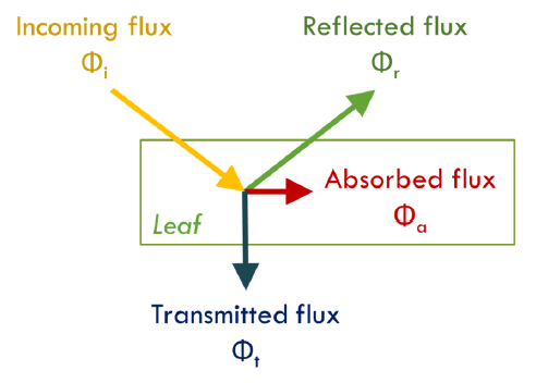
Figure 1 Dynamics of the luminous flux incoming on a leaf
Balance between reflection, absorption and transmission depend on the characteristics of the plant. This balance is expressed by different values. For example, reflectance (\(R\)) is a value between 0 and 1 calculated as follows:
\[ \quad\text{(Eq. 1)}\quad R = \frac{\phi_{r}}{\phi_{i}} \]
Where \(\phi_{r}\) stands for reflected flux and \(\phi_{i}\) for incoming flux. In the same way, absorbance (\(A\)) corresponds to the ratio between absorbed flux and incoming flux.
Incoming solar radiation flux is composed of different wavelengths. Photosynthetically active radiation (PAR), designates the spectral range of solar radiation (usually from 400 to 700 nanometers) that photosynthetic organisms are able to absorbate and use in the process of photosynthesis. PAR is usually quantified as a photon flux (μmol photons per m-2.s-1).
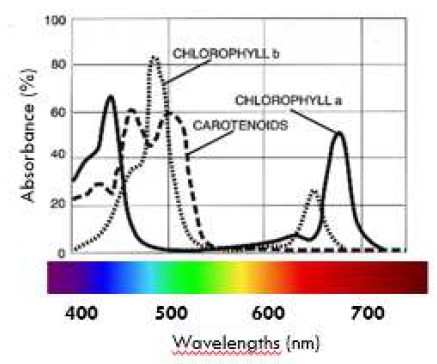
Figure 2 Absorbance spectrum of the main plant pigments (adapted from Whitmarsh and Govindjee)
As can be seen in Figure 2, the absorption spectrum of plants is high in the red (around 650nm) and then rapidly decreases in the infrared (above 700nm). Conversely, plants will have a higher relative reflectance in the infrared than in the red. Normalized Difference Vegetation Index (NDVI) calculation is based on the relative difference in reflectance between these two wavelengths:
\[ \quad\text{(Eq. 2)}\quad NDVI = \frac{R_{NIR}-R_{Red}}{R_{NIR}+R_{Red}} \]
Where \(R_{Red}\) is the reflectance in the red wavelength and \(R_{NIR}\) the reflectance in the near infra-red.
As reflectances vary between 0 and 1, the NDVI itself thus varies between -1 and +1. It may be a practical advantage compared to the simple ratio (Near infrared/Red), which is always positive but has a mathematically infinite range (0 to infinity).
Reflectances are measured by spectral sensors, which simultaneously measure this value for several wavelengths (about ten for multispectral sensors, a hundred for hyperspectral sensors, thousands for ultraspectral sensors). We will discuss below Sentinel-2 multispectral sensors.
2. Download Sentinel-2 multispectral aerial images
The Sentinel program of the ESA gathers several missions that focus on different aspects of Earth observation such as atmospheric, oceanic, and land monitoring. Vegetation monitoring is mainly carried out with the Sentinel-2 mission. Sentinel-2 is composed of two polar-orbiting satellites providing high-resolution optical imagery.
On the data download interface of the Copernicus website, you need to create and account and register, then follow this procedure:
- Manually search the area of interest on the map
- Once the area is located, click on the “Switch to area mode” icon at the top right of the map and then select the area of interest
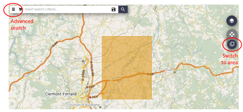
Figure 3 Selection of the area of interest on the Copernicus interface
- From the Advanced search criteria, select:
- Sensing period;
- Sentinel 2 mission (for multispectral aerial images);
- Do not select any particular satellite (keep both S2A and S2B for more results);
- Choose images with a low Cloud Cover rate (e.g. [0 TO 10], for a cloud cover rate below 10%);
- Product type: MSI is for multispectral images. Then choose the data that end with 2A (for Level 2A), which corresponds to the reflectance at the bottom of the atmosphere (including atmospheric correction), while the data ending with 1C corresponds to the reflectance at the top of the atmosphere.
- Until March 2018: choose 2Ap (pilot version);
- After March 2018: choose 2A (operational version).
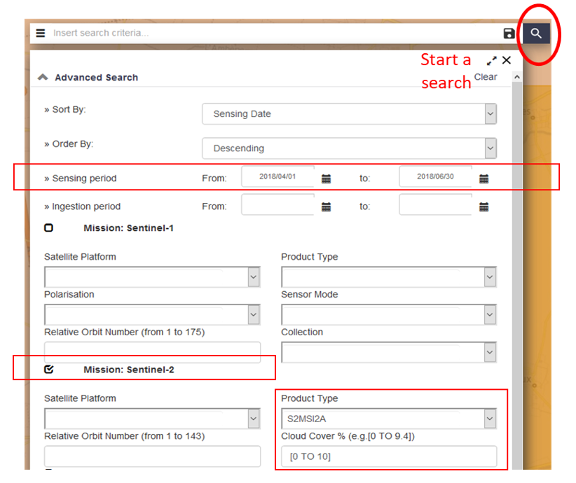
Figure 4 Definition of a request with Advanced search criteria
Start a search and look through the results. Before downloading the data, you may check cloud coverage and image extent. Each file size is approximately 600MB (tiles of 100km*100km).
3. Create a NDVI map with QGIS
The following procedure has been performed with QGIS 3.6, but is easily reproducible with previous versions.
Unzip the downloaded file. Inside it, look for the “Granule” folder, then the “IMG_DATA” folder. It contains three sub-folders “R10m”, “R20m” and “R60m” which correspond to three different resolutions (from 10m * 10m to 60m * 60m per pixel).
Sentinel 2 provides reflectance measurements for 13 wavelengths, but only four of them are available at the 10m resolution:
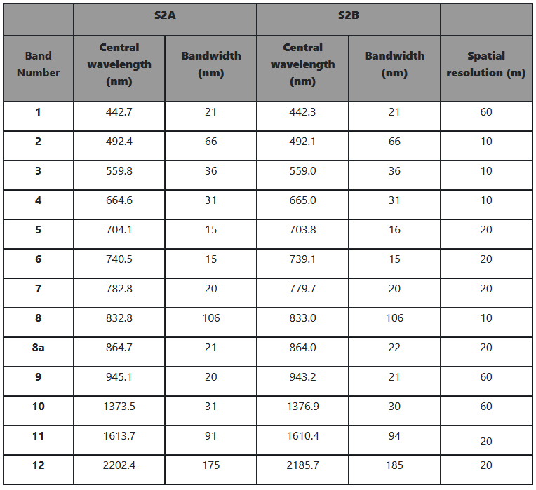
Figure 5 Spectral bands for Sentinel-2 sensors (Source: sentinel.esa.int)
As shown in Table 1, Sentinel-2 sensors have 4 native 10m bands: B02 (blue), B03 (green), B04 (red) and B08 (near infrared). As only bands B02 and B08 are required for NDVI calculation, maps can be produced with a resolution of 10*10m (however, keep in mind that Sentinel-2 images have a positioning uncertainty of approximately 10m, which must also be taken into account when overlaying several images for example).
For the next steps, we will focus on the data in the “R10” folder. In QGIS, open the two rasters whose names end with *…_B04_10m* and *…_B08_10m* (red and near infrared reflectance, respectively). You may also open the “True Colors Index” raster (name ending with …TCI_10m) to check for cloud cover for example.
Then, in the “Raster” menu, open the “Raster Calculator”. Enter the name of the layer to be saved, ending with *…_NDVI*. Following \(Eq. 2\), the NDVI formula to be entered is:
\[ \quad\text{(Eq. 3)}\quad NDVI = \frac{B08-B04}{B08+B04} \]
Where \(B04\) is the reflectance in the red wavelength and \(B08\) the reflectance in the near infra-red.
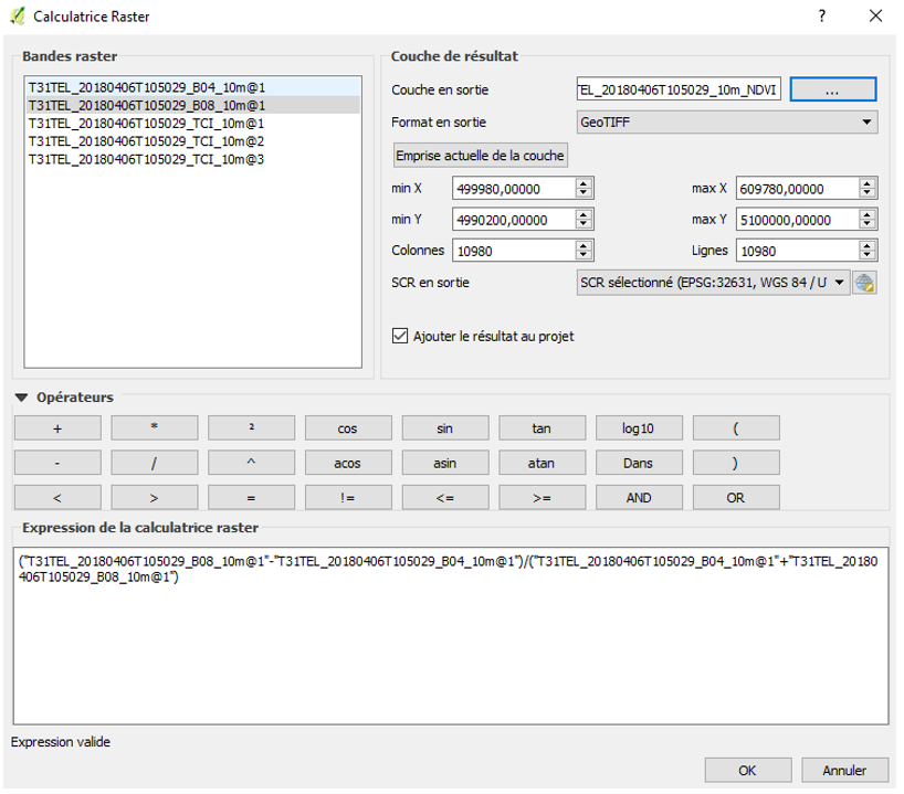
Figure 6 Compute NDVI with raster calculator
We may now display our NDVI map with an appropriate color scale (right click on the raster name > Properties > Style). Also, in order to display the contrasts more clearly for one field of interest, it is appropriate to cut the raster according to the field boundaries with the « Clip raster with polygon » function.
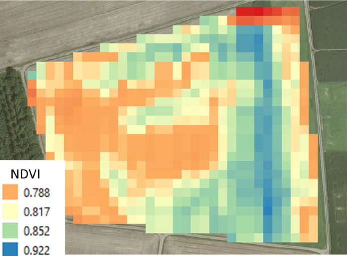
Figure 7 Within-field variability of NDVI for a wheat field (April 2018)
4. Processing multiple dates
The above procedure works for a limited number of dates. If you want to process multiple dates and/or a large area of interest, it is better to work with an API, which allows you to process queries without having to download all the images.For example, for the article mentioned above, we used the Google Earth Engine platform to extract an average NDVI per field for France. Yet, having manually processed an NDVI map first allows for a better understanding of APIs later on.
I will present the processing of NDVI maps with the Google Earth Engine in a future post.