In this post, we will see how to create an interactive graph with the {ggiraph} package from David Gohel. For this, we will use FAO Stats data to highlight the main coffee growers in the world.
1. Data preparation
For this tutorial, we will also need the {tidyverse} libraries for data preparation. Let’s start by loading the data that are available online in one of my Github repo.
# Load libraries
library(tidyverse)

# Load data: crop harvested areas in 2018
data <- readr::read_csv(
  'https://raw.githubusercontent.com/BjnNowak/playground/main/data/all_crops_area.csv'
)

head(data)
## # A tibble: 6 x 14
## `Domain Code` Domain `Area Code (FAO~ Area `Element Code` Element
## <chr> <chr> <dbl> <chr> <dbl> <chr>
## 1 QCL Crops and liv~ 2 Afghan~ 5312 Area har~
## 2 QCL Crops and liv~ 2 Afghan~ 5312 Area har~
## 3 QCL Crops and liv~ 2 Afghan~ 5312 Area har~
## 4 QCL Crops and liv~ 2 Afghan~ 5312 Area har~
## 5 QCL Crops and liv~ 2 Afghan~ 5312 Area har~
## 6 QCL Crops and liv~ 2 Afghan~ 5312 Area har~
## # ... with 8 more variables: Item Code (FAO) <dbl>, Item <chr>,
## # Year Code <dbl>, Year <dbl>, Unit <chr>, Value <dbl>, Flag <chr>,
## # Flag Description <chr>Then, we will keep only the 10 countries with the most important surfaces cultivated in coffee (by decreasing order).
# Keep 10 countries with bigger coffee area
clean <- data%>%
  filter(Item=="Coffee, green")%>%
  arrange(-Value)%>%
  head(10)%>%
  # Convert area to Mha
  mutate(Surface=Value/1000000)%>%
  select(Country=Area,Surface)
2. From static to interactive plot
We will now create the “static” version of the graph that we want: a barplot showing the cultivated areas per country.
# Make static plot
ggplot(data=clean,aes(
    y=fct_reorder(Country,Surface),
    x=Surface))+
  geom_col(fill="chocolate4")+
  labs(
    title="Main coffee growers",
    x="Surface (Mha)",
    y=""
  )+
  theme_light()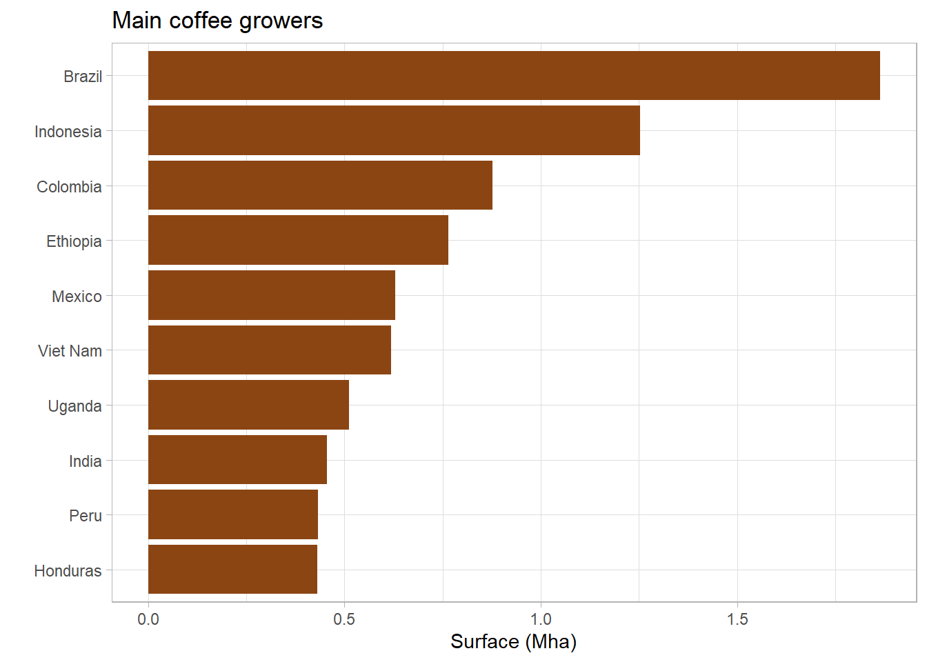
With {ggraph}, it is then very easy to convert a static graph into an interactive version. There are two things to change:
- Add _interactive to the geom_ you are using
- Specify the label you want to display with the tooltip attribute in the aes()
library(ggiraph)

# Plot with interactive geom_
plot1<-ggplot(data=clean,aes(
    y=fct_reorder(Country,Surface),
    x=Surface))+
  geom_col_interactive(
    # Specify label in aes()
    # with tooltip
    aes(tooltip=Surface),
    fill="chocolate4"
  )+
  labs(
    title="Main coffee producers",
    x="Surface (Mha)",
    y=""
  )+
  theme_light()
We may then display the interactive plot as follows:
# Create a girafe object
i1 <- ggiraph::girafe(
  ggobj = plot1
)

i1
3. Customize labels
The first step of customization will be to personalize the general aspect of the labels thanks to a small css script that we can then add when creating the ggirafe object.
# css for general label
custom_css <- "
  background-color:cornsilk;
  color:black;
  padding:10px;
  border-radius:5px;"

i1b <- ggiraph::girafe(
  ggobj = plot1,
  # Add custom css to girafe object
  options = list(opts_tooltip(css = custom_css))
)

i1b
But the labels are not very clear and only give the total area cultivated in coffee, without specifying the unit for example. We will now create labels with a more complete and detailed text.
To do this, before creating our plot, we will add a new column in our data set that will contain the text we want to display, specifying with HTML and css code the presentation we want.
# Create custom label
clean_label <- clean %>%
  # Round area harvested (2 decimals only)
  mutate(Surf_round = round(Surface,2))%>%
  # Add country rank
  mutate(Rank = row_number())%>%
  # Add custom label
  mutate(lab=glue::glue(
    "<body><span style='font-weight: 900;'>{Rank}. {Country}</span>
    <br>{Surf_round} Mha </body>"))
We are now ready to create a new plot using this new label.
# Make plot with new new dataset
# and tooltip with new label
plot2<-ggplot(data=clean_label,aes(
  y=fct_reorder(Country,Surface),
  x=Surface))+
  geom_col_interactive(
    aes(tooltip=lab),
    fill="chocolate4"
  )+
  labs(
    title="Main coffee producers",
    x="Surface (Mha)",
    y=""
  )+
  theme_light()

i2 <- girafe(
  ggobj = plot2,
  options = list(opts_tooltip(css = custom_css))
)

i2
4. Interactive map of most cultivated crops
To finish this tutorial, here is an example of an intercative map created with the same method. This map shows the most cultivated crop for each country (by harvested area). The most common crops are mainly cereals (wheat, maize, rice, barley and millet), with also a strong share of soybeans in the Americas. Beyond these main crops, some countries are specialized in other crops (such as coffee or oil palm).
You may find the full code for this example here.
References
Goehel, D., ggiraph makes ‘ggplot’ graphics interactive.