1. Get the data

For this example, we will use the data of week 33 (year 2021) of Tidy Tuesday, about investments on infrastructure in the US from 1947 to 2017 (Bennett et al., 2020).

# Load data 
chain_investment <- readr::read_csv('https://raw.githubusercontent.com/rfordatascience/tidytuesday/master/data/2021/2021-08-10/chain_investment.csv')

head(chain_investment)

## # A tibble: 6 x 5
##   category                   meta_cat            group_num  year gross_inv_chain
##   <chr>                      <chr>                   <dbl> <dbl>           <dbl>
## 1 Total basic infrastructure Total infrastructu~         1  1947          73279.
## 2 Total basic infrastructure Total infrastructu~         1  1948          83218.
## 3 Total basic infrastructure Total infrastructu~         1  1949          95760.
## 4 Total basic infrastructure Total infrastructu~         1  1950         103642.
## 5 Total basic infrastructure Total infrastructu~         1  1951         102264.
## 6 Total basic infrastructure Total infrastructu~         1  1952         107278.

2. Single area plot

There’s a lot of information in this dataset, we’re going to start looking at the breakdown of investment between the three main domains: basic, social and digital.

# Load extensions for data handling
library(tidyverse)

# Filter for main domains only
main <- chain_investment%>%
  filter(group_num==1)%>%    # Filter thanks to "group_num" attribute                     
  mutate(lab=case_when(      # New column with simpler names
    category=="Total basic infrastructure"~"Basic",
    category=="Total digital infrastructure"~"Digital",
    category=="Total social infrastructure"~"Social"
  ))

head(main)

## # A tibble: 6 x 6
##   category               meta_cat          group_num  year gross_inv_chain lab  
##   <chr>                  <chr>                 <dbl> <dbl>           <dbl> <chr>
## 1 Total basic infrastru~ Total infrastruc~         1  1947          73279. Basic
## 2 Total basic infrastru~ Total infrastruc~         1  1948          83218. Basic
## 3 Total basic infrastru~ Total infrastruc~         1  1949          95760. Basic
## 4 Total basic infrastru~ Total infrastruc~         1  1950         103642. Basic
## 5 Total basic infrastru~ Total infrastruc~         1  1951         102264. Basic
## 6 Total basic infrastru~ Total infrastruc~         1  1952         107278. Basic

We are ready to plot our first area plot, with {ggplot2} and geom_area().

ggplot(
  data=main,
  aes(x=year,y=gross_inv_chain,fill=lab)      # Choose newly created lab column for fill
  )+
  geom_area()+
  labs(
    title = "Evolution of investment on US infrastructures",
    x="Year",
    y="Investment (millions of 2012 $)"
  )+
  theme_minimal()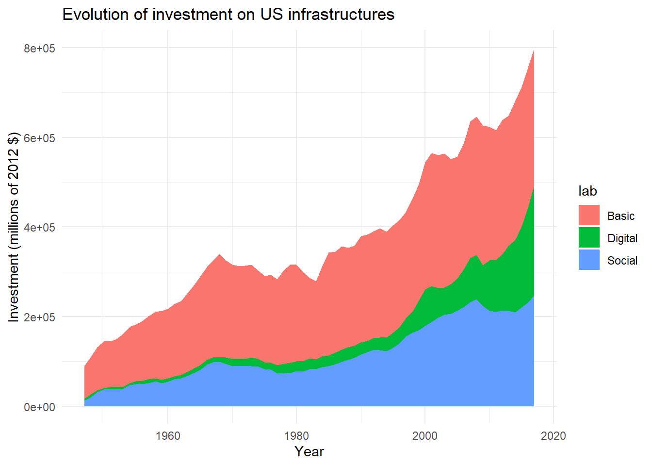

For more clarity, we will reorder factors from highest to lowest investments.

# Reorder factors
main$lab<-factor(
  main$lab,
  c(
    "Digital",
    "Social",
    "Basic"
  ))

# Plot again
ggplot(
  data=main,
  aes(x=year,y=gross_inv_chain,fill=lab)   
  )+
  geom_area()+
  labs(
    title = "Evolution of investment on US infrastructures",
    x="Year",
    y="Investment (millions of 2012 $)"
  )+
  theme_minimal()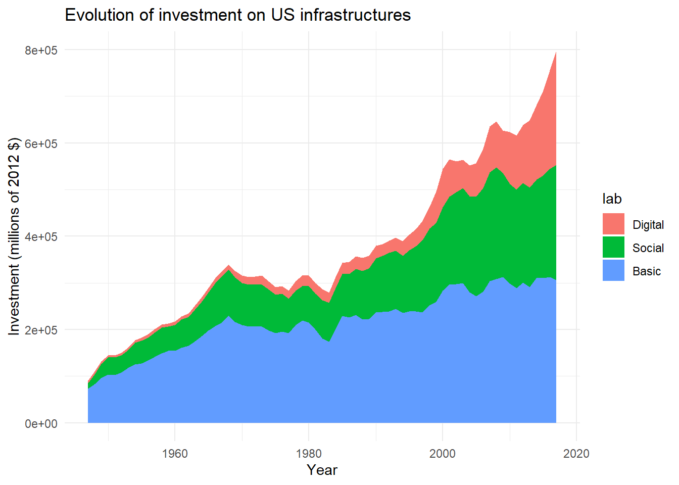

Now we want to add the names of the factors directly to the right of the graph, so that we don’t have to add a legend. To do this, we will start by creating a new data frame that will contain the value taken by each factor for the last year (2017), and sum these values from the first factor (Basic) to the last factor (Digital), so we can use these values as y positions for our legend labels.

final<-main%>%
  filter(year=="2017")%>%              # Keep only 2017 value
  arrange(desc(lab))%>%                # Inverse factor order (first is at the bottom of plot)
  mutate(                              # Create new column ypos and
    ypos=cumsum(gross_inv_chain)       # fill with cumulative sum of invest for 2017
  )                                     

final

## # A tibble: 3 x 7
##   category           meta_cat       group_num  year gross_inv_chain lab     ypos
##   <chr>              <chr>              <dbl> <dbl>           <dbl> <fct>  <dbl>
## 1 Total basic infra~ Total infrast~         1  2017         306038. Basic 3.06e5
## 2 Total social infr~ Total infrast~         1  2017         247348. Soci~ 5.53e5
## 3 Total digital inf~ Total infrast~         1  2017         245817  Digi~ 7.99e5

Then, we can use this data frame to position directly the labels on the plot, with geom_text().

ggplot(
  data=main,
  aes(x=year,y=gross_inv_chain,fill=lab)   
  )+
  geom_area()+
  labs(
    title = "Evolution of investment on US infrastructures",
    x="Year",
    y="Investment (millions of 2012 $)"
  )+
  geom_text(
    data=final,              # Different data than the main plot
    aes(y=ypos,label=lab),   # y and lab in the aes() (change between labels)
    x=2017                   # x is the same for all labels
  )+
  theme_minimal()

As you can see, this first layout is not optimal. But we can now modify the code to improve the labels positioning

ggplot(
  data=main,
  aes(x=year,y=gross_inv_chain,fill=lab)   
  )+
  geom_area()+
  labs(
    title = "Evolution of investment on US infrastructures",
    x="Year",
    y="Investment (millions of 2012 $)"
  )+
  geom_text(
    data=final,              
    aes(
      y=ypos-150000,         # Decrease label y position 
      label=lab),   
    x=2018, 
    hjust=0                  # Left align text
  )+
  scale_x_continuous(
    limits=c(1947,2022),     # Expand x axis to leave space for labels
    breaks=c(1950,1980,2010)
  )+
  guides(
   fill=FALSE                # No need for fill legend anymore !
  )+
  theme_minimal()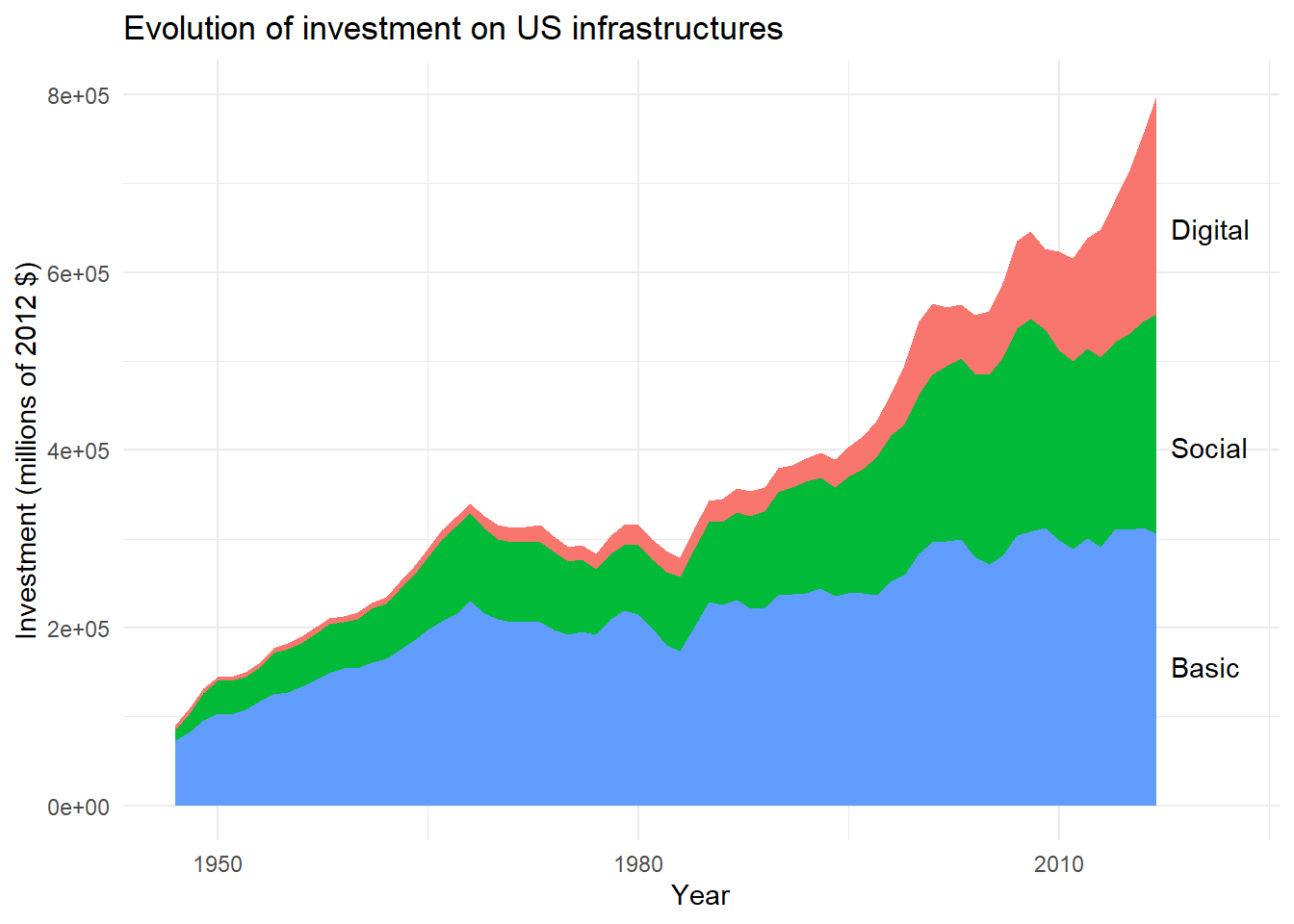

This is already better. But, to make this plot even easier to read, we will finish this one by associating the same colors for our filled areas and matched labels.

# Create color palette
pal<-c("#0F4C5C","#E36414","#9A031E")

# Specify color palette with a new column inside main
main<-main%>%
  mutate(
    col_lab=case_when(
      lab=="Basic"~"#0F4C5C",
      lab=="Social"~"#E36414",
      lab=="Digital"~"#9A031E"
    ))

Now that the color palette is created, we may use it inside ggplot() for both fill and color arguments.

ggplot(
  data=main,
  aes(x=year,y=gross_inv_chain,fill=lab)   
  )+
  geom_area()+
  labs(
    title = "Evolution of investment on US infrastructures",
    x="Year",
    y="Investment (millions of 2012 $)"
  )+
  geom_text(
    data=final,              
    aes(
      y=ypos-150000,         
      label=lab,
      color=lab            # Add color inside the aes()
    ),   
    x=2018, 
    hjust=0                  
  )+
  scale_fill_manual(       # Specify fill palette
    breaks=main$lab,values=main$col_lab
  )+
  scale_color_manual(      # Same palette for color
    breaks=main$lab,values=main$col_lab
  )+
  scale_x_continuous(
    limits=c(1947,2022),     
    breaks=c(1950,1980,2010)
  )+
  guides(
   fill=FALSE,
   color=FALSE             # Hide color legend
  )+
  theme_minimal()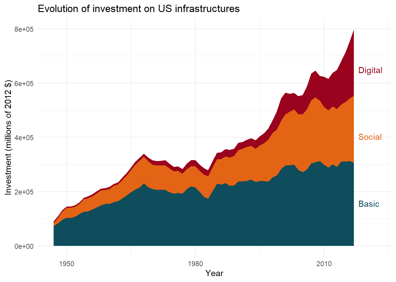

3. Faceted area plots

The workflow presented above may be adapted to faceted area plots. We will see this by detailing the categories included in each of the three main areas. Let’s start by selecting the sub-categories, with just a few modifications to shorten the name of the longest categories.

sub <- chain_investment%>%
  filter(
    group_num==4|   # Basic
    group_num==17|  # Social
    group_num==22   # Digital
  )%>%
  mutate(lab=case_when(     # Create new column with shortest names
    category=="Conservation and development"~"Conservation",
    category=="Private computers in NAICS 515, 517, 518, and 519"~"Computers",
    category=="Private software in NAICS 515, 517, 518, and 519"~"Software",
    category=="Private communications equipment in NAICS 515, 517, 518, and 519"~"Com. equipment",
    category=="Private communications structures"~"Com. structures",
    TRUE~category
  ))

We may now produce faceted area plots.

ggplot(
  data=sub,
  aes(x=year,y=gross_inv_chain,fill=lab)   
  )+
  geom_area()+
  facet_wrap(
    ~meta_cat,
    ncol=1,
    strip.position = "top"
  )

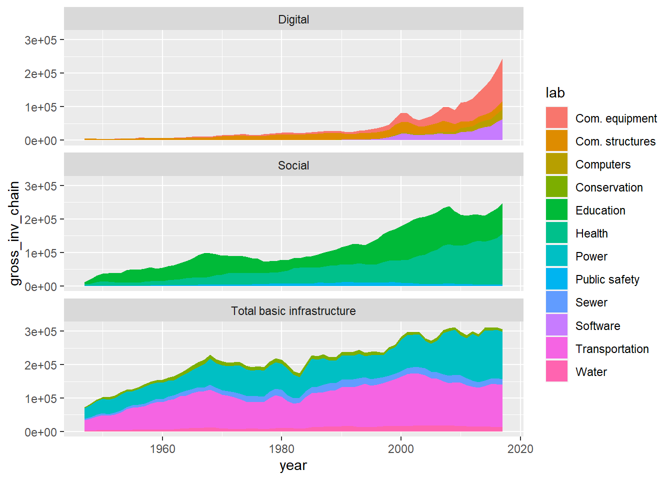
With this number of categories, the advantage of labels directly in the graph is even more important. To do this, we will use the same procedure as in the previous section, but this time we will specify that the sums must be realized by major domains (basic, social or digital). To do so, we will use group_by().

final_sub<-sub%>%
  filter(year=="2017")%>%
  group_by(group_num)%>%    # Group by major fields before cumulative sums
  arrange(desc(category))%>%
  mutate(ypos=cumsum(gross_inv_chain))%>%
  ungroup()

We may now use this data frame to position the labels with geom_text().

ggplot(
  data=sub,
  aes(x=year,y=gross_inv_chain,fill=lab)   
  )+
  geom_area()+
  facet_wrap(
    ~meta_cat,
    ncol=1,
    strip.position = "top"
  )+
  geom_text(
    data=final_sub,
    aes(y=ypos-20000,label=lab,color=lab),
    x=2018,hjust=0,
    fontface="italic"
  )+
  scale_x_continuous(limits = c(1947,2030),breaks=c(1950,1970,1990,2010) )+
  guides(
    fill=FALSE,
    color=FALSE
  )+
  labs(
    title = "Evolution of investment on US infrastructures",
    x="Year",
    y="Investment (millions of 2012 $)"
  )+
  theme_minimal()

With so many labels, they are not easy to read. To improve readability, we will decrease the text size. We will also use the {ggrepel} extension to try to optimize the position of the labels, by replacing geom_text() with geom_text_repel().

library(ggrepel)          # Load extension

facet<-ggplot(
  data=sub,
  aes(x=year,y=gross_inv_chain,fill=lab)   
  )+
  geom_area()+
  facet_wrap(
    ~meta_cat,
    ncol=1,
    strip.position = "top"
  )+
  geom_text_repel(        # Replace geom_text()
    data=final_sub,
    aes(y=ypos-20000,label=lab,color=lab),
    direction='y',        # Repel on y-axis (align on x-axis)
    x=2018,hjust=0,
    size=3,               # Decrease size
    fontface="italic"
  )+
  scale_x_continuous(limits = c(1947,2030),breaks=c(1950,1970,1990,2010) )+
  guides(
    fill=FALSE,
    color=FALSE
  )+
  labs(
    title = "Evolution of investment on US infrastructures",
    x="Year",
    y="Investment (millions of 2012 $)"
  )+
  theme_minimal()

facet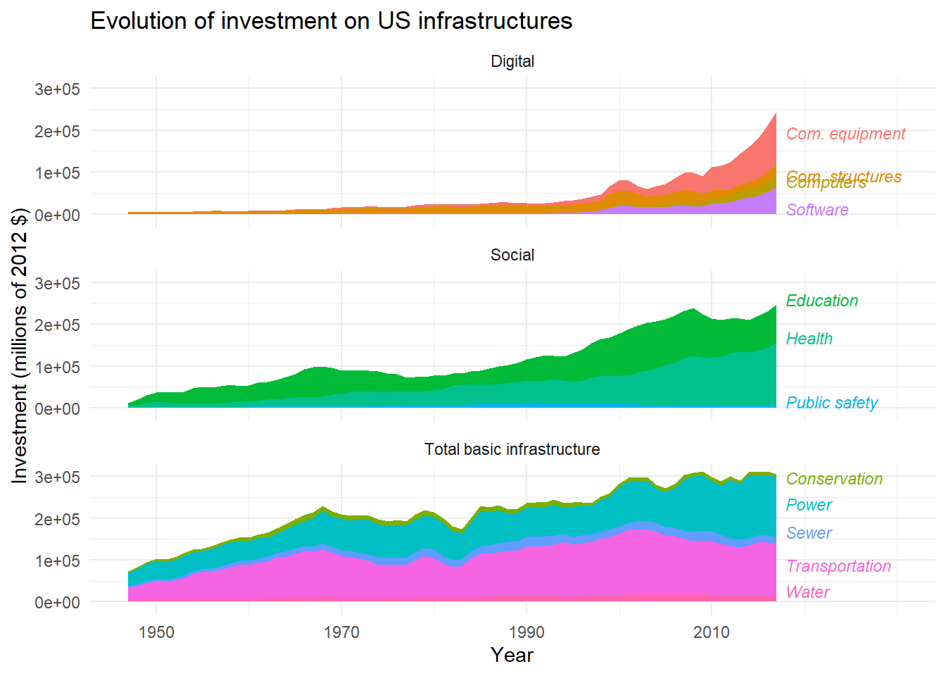

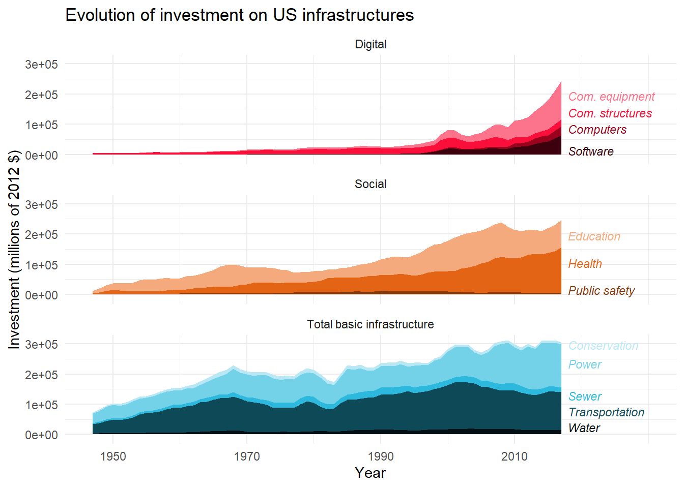
As before, we may also customize the color palette.

# Create color palettes based on 
# color gradients of former legend

pal_basic <- c(
  "#030F12",
  "#0E4958",
  "#2CB9DD",
  "#73D1E8",
  "#B9E8F4"
)

pal_social <- c(
  "#83390B",
  "#E36414",
  "#F4AA7C"
)

pal_digital <- c(
  "#3C010C",
  "#9A031E",
  "#FA0F3A",
  "#FC738C"
)

# Add color palette to data
sub<-sub%>%
  mutate(col_lab=case_when(
    lab=="Water"~pal_basic[1],
    lab=="Transportation"~pal_basic[2],
    lab=="Sewer"~pal_basic[3],
    lab=="Power"~pal_basic[4],
    lab=="Conservation"~pal_basic[5],
    lab=="Public safety"~pal_social[1],
    lab=="Health"~pal_social[2],
    lab=="Education"~pal_social[3],
    lab=="Software"~pal_digital[1],
    lab=="Computers"~pal_digital[2],
    lab=="Com. structures"~pal_digital[3],
    lab=="Com. equipment"~pal_digital[4]
  ))

# Add color to plots
facet+  
  scale_fill_manual(       # Specify fill palette
    breaks=sub$lab,values=sub$col_lab
  )+
  scale_color_manual(      # Same palette for color
    breaks=sub$lab,values=sub$col_lab
  )

4. Combine plots

Finally, we can combine both plots using {patchwork} or {cowplot}, as in the example below, so the legend of one plot becomes the title of other plots.

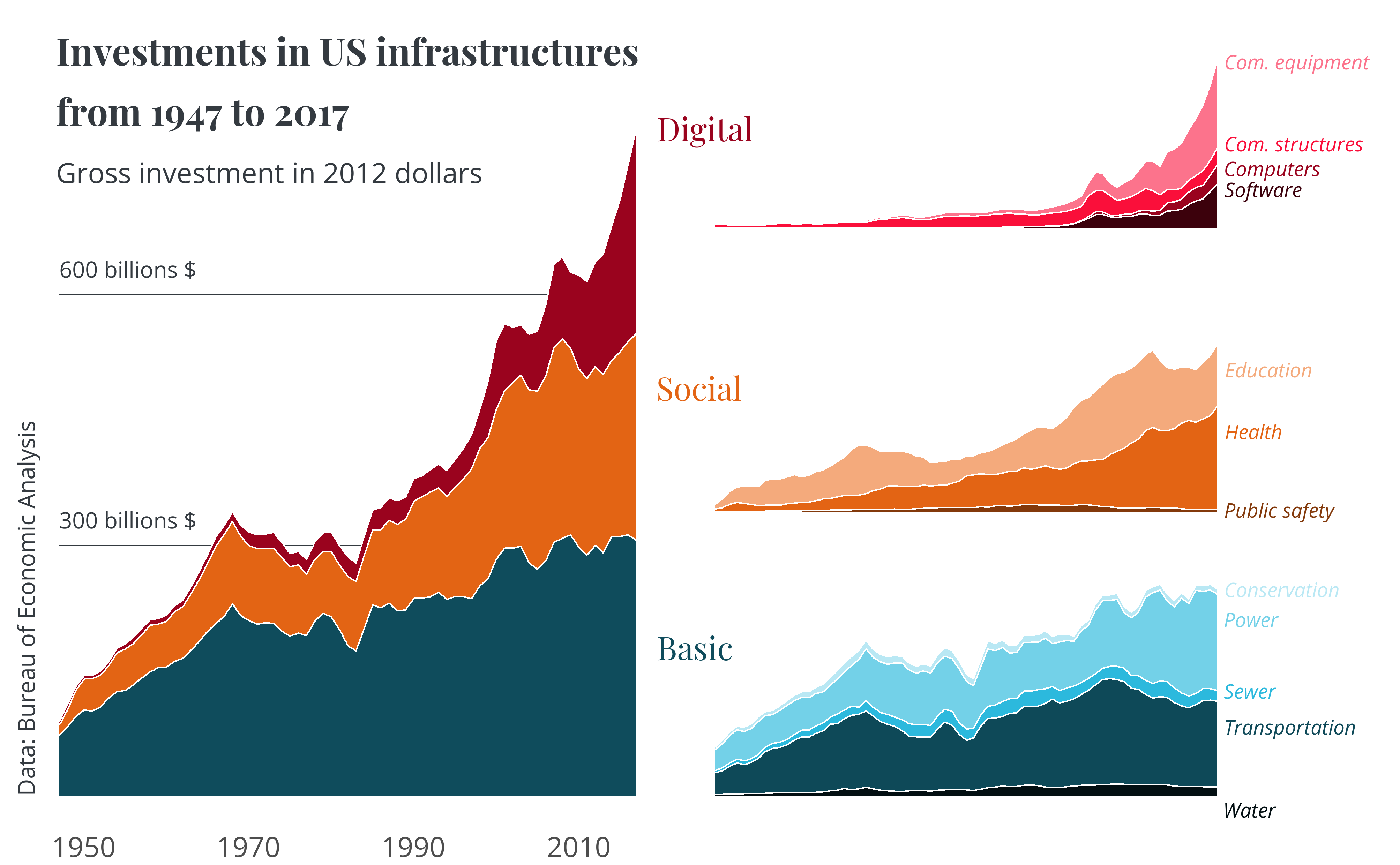
You may find the full code for this example here.

References

• Bennett J. et al., 2020 Measuring Infrastructure in the Bureau of Economic Analysis National Economic Accounts
• Mock T., Tidy Tuesday
• Scherer C., A Quick How-to on Labelling Bar Graphs in ggplot2